Search
- Often not given an algorithm to solve a problem
- Only specification of what is a solution
- We have to search for a solution
- We can do so by exploring a directed graph that represents the state space of our problem
- Sometimes the graph is literal
- Nodes may represent actual locations in space
- Edges represent the distance between them
- Sometimes the graph is implicit
- Nodes represent states
- Edges represent state transitions
Directed Graphs
- A graph consists of a set
of nodes and a set of ordered pairs of nodes, called arcs or edges - Node
is a neighbor of if there is an arc from to - A path is a sequence of nodes
such that - Often there is a cost associated with arcs and the cost of a paths is the sum of the costs of the arcs in the path
A Search Problem
- A search problem is defined by:
-
- A set of states
- An initial state
- Goal states
- a boolean function which tells whether a given state is a goal state
- A successor/neighbor function
- an action which takes us from one state to other states
- A cost associated with each action
A solution to the problem is a path from the start state to a goal state
- optionally with the smallest cost
Graph Searching
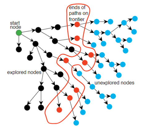
Generic search algorithm:
- Given a graph, start nodes, and goal nodes, incrementally explore paths from the start nodes
- Maintain a frontier of paths from the start node that have been explored
- As search proceeds, the frontier expands into the unexplored nodes until a goal node is encountered
- The way in which the frontier is expanded defines the search strategy
Graph Search Algorithm
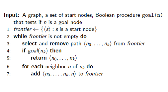
- We assume that after the search algorithm returns an answer, it can be asked for more answers and the procedure continues
- The neighbors define the graph structure
- Which value is selected from the frontier and how the new values are added to the frontier at each stage defines the search strategy
- Goal defines what is a solution
Uniformed (blind) Search
Depth-First Search
- DFS treats the frontier as a stack
- It always selects the last element added to the frontier
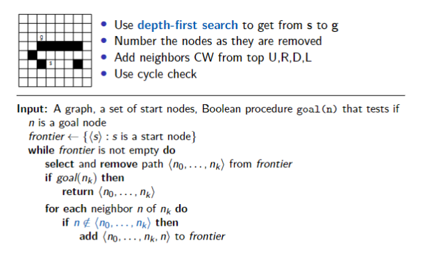
Cycle Checking
- A searcher can prune a path that ends in a node already on the path
- We will assume that this check can be done via hashing in constant time
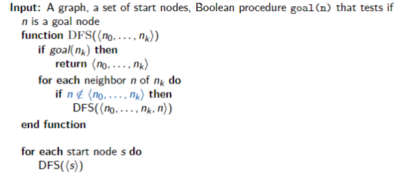
Implementation of DFS
Properties of DFS
Useful Quantities
- b is the branching factor
- m is the maximum depth of the search tree
- d is the depth of the shallowest goal node
Properties
- Space Complexity: size of frontier in worst case
- Time Complexity: number of nodes visited in worst case
- Completeness: does it find a solution when one exists?
- No, will get stuck in an infinite path
- Optimality: if solution found, is it the one with the least cost?
- No, it pays no attention to the costs and makes no guarantee on the solution’s quality
When should we use DFS?
Useful when:
- Space is restricted
- Many solutions exist, perhaps with long paths
DFS is a poor method when: - There are infinite paths
- Solutions are shallow
- There are multiple paths to a node
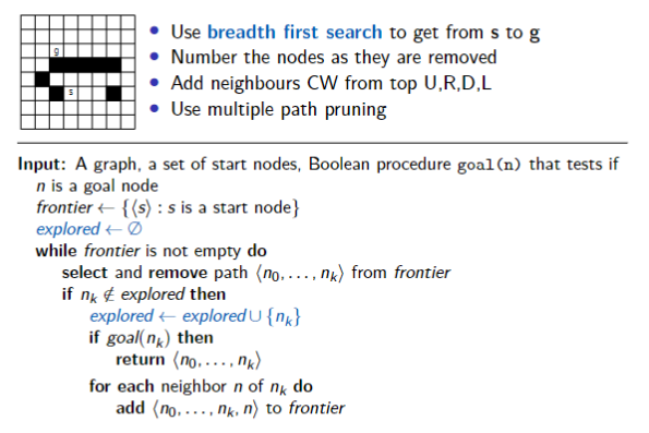
Breadth-First Search
- BFS treats the frontier as a queue
- It always selects the earliest element added to the frontier
Multiple-Path Pruning
Prune a path to node
- subsumes a cycle check because the current path is a path to the node
- Need to store all nodes it has found paths to
- Want to guarantee that an optimal solution can still be found
Implementation
Properties of DFS
Properties
- Space Complexity: size of frontier in worst case
- Time Complexity: number of nodes visited in worst case
- Completeness: does it find a solution when one exists?
- Yes, explores the tree level by level until it finds a goal
- Optimality: if solution found, is it the one with the least cost?
- No, guaranteed to find the shallowest goal node
When should we use BFS
Useful when:
- Space is not a concern
- We would like a solution with the fewest arcs
Poor method when: - All the solution are deep in the tree
- The problem is large and the graph is dynamically generated
Iterative-Deepening Search
Combine the best of BFS and DFS
- For every depth limit, perform DFS until the depth limit is reached
Properties
Properties
- Space Complexity: size of frontier in worst case
- similar to DFS
- Time Complexity: number of nodes visited in worst case
- Same as BFS
- Completeness: does it find a solution when one exists?
- Yes, explores the tree level by level until it finds a goal
- Same as BFS
- Optimality: if solution found, is it the one with the least cost?
- No, guaranteed to find the shallowest goal node
- Same as BFS
Lowest-Cost-First Search
Sometimes there are costs associated with arcs
- The cost of a path is the sum of the costs of its arcs
At each stage, LCFS selects a path on the frontier with lowest cost - The frontier is a priority queue ordered by path cost
- It finds a least-cost path to a goal node
- When arc costs are equal
BFS - Still uniformed/blind search (does not take the goal into account)
Properties
- Space Complexity: size of frontier in worst case
- Exponential
- Time Complexity: number of nodes visited in worst case
- Exponential
- Completeness: does it find a solution when one exists?
- Yes, if branching factor is finite and cost of each edge is strictly positive
- Optimality: if solution found, is it the one with the least cost?
- Yes, if branching factor is finite and cost of each edge is strictly positive
Dijkstra’s Algorithm
Variant of LCFS with a kind of multiple-path pruning
- Like LCFS, frontier is stored in priority queue, sorted by cost
- For every node in the graph, we keep track of the lowest cost to reach it so far
- If we find a lower cost path to a node, we update that value
- May require re-sorting the priority queue
- An example of dynamic programming because it trades space (store value for each node) for time (find the shortest path faster)
Heuristic Search
Idea: don’t ignore the goal when selecting paths
- Often there is extra knowledge that can be used to guide the search: heuristic
is an estimate of the cost of the shortest path from node to a goal node - uses only readily obtainable information about a node
- computing the heuristic must be much easier than solving the problem
can be extended to paths: is an underestimate if there is no path from to a goal that has path length less than
- If the nodes are points on a Euclidean plane and the cost is the distance, we can use the straight-line distance from
to the closest goal as the value of - If the nodes are locations and cost is time, we can use the distance to a goal divided by the maximum speed
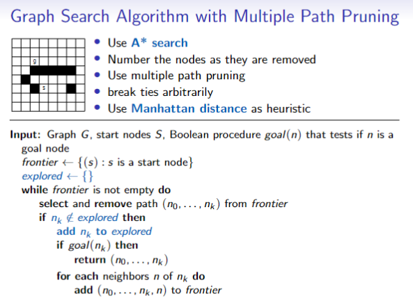
- If nodes are locations on a grid and cost is distance, we can use the Manhattan distance
- distance by taking horizontal and vertical moves only
Greedy Best-First Search
Idea: select the path whose end is closest to a goal according to the heuristic function
- Best-first search selects a path on the frontier with minimal
-value - It treats the frontier as a priority queue ordered by
Implementation

Properties
- Space and Time complexities
- Both exponential
- Completeness and Optimality
- No, GBFS is not complete
- It could be stuck in a cycle
- No, GBFS is not optimal
- It may return a sub-optimal path first
- No, GBFS is not complete
Heuristic Depth-First Search
Idea: Do a DFS, but add paths to the stack ordered according to
- Locally does a best-first search, but aggressively pursues the best looking path
- Even if it ends up being worse than one higher up
- Same properties as regular depth-first search
- Is often used in practice
Implementation

A* Search
Uses both path cost and heuristic values
: the cost of path estimates the cost from the end of to a goal - Let
; estimates the total path cost of going from a start node to a goal via

A* is a mix of lowest-cost-first and best-first search - It treats the frontier as a priority queue ordered by
- It always selects the node on the frontier with the lowest estimated distance from the start to a goal node constrained to go via the node
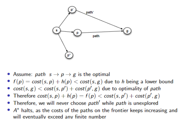
Admissibility of A*
If there is a solution, A* always finds an optimal solution - the first to a goal selected - if
- The branching factor is finite
- Arc costs are bounded above zero
is a lower bound on the length of the shortest path from to a goal node
Proof
Implementation
Properties
Space and Time Complexities
- Both are exponential
Completeness and Optimality - Yes and Yes
- assuming the heuristic function is admissible, the branching factor is finite, and arc costs are bounded above zero
Optimally Efficient
Among all optimal algorithms that start from the same start node and use the same heuristic, A* expands the fewest nodes
- No algorithm with the same information can do better
- A* expands the minimum number of nodes to find the optimal solution
- Intuition for proof:
- any algorithm that does not expand all nodes with
run the risk of missing the optimal solution
- any algorithm that does not expand all nodes with
Constructing an Admissible Heuristic
- Define a relaxed problem by simplifying or removing constraints on the original problem
- Solve the relaxed problem without search
- The cost of the optimal solution to the relaxed problem is an admissible heuristic for the original problem
Desirable heuristic properties
- We want a heuristic to be admissible
- A* is optimal
- We want a heuristic to have higher values
- The close
is to , the more accurate is
- The close
- Prefer a heuristic that is very different for different states
should help us choose among different paths - If
is close to constant, it’s not useful
Dominating Heuristic
Given heuristics
If
Multiple-Path Pruning & Optimal Solutions
- Remove all paths from the frontier that use the longer path
- Change the initial segment of the paths on the frontier to use the shorter path
- Ensure this doesn’t happen: make sure that the shortest path to a node is found first
- lowest-cost-first-search
Multiple-Path Pruning & A*
Suppose path
because was selected before because the path to via is shorter (by assumption)
You can ensure this doesn’t occur by letting
Monotone Restriction
Heuristic function
- Monotone heuristic functions are also called consistent
is the heuristic estimate of the path cost from to - The heuristic estimate of the path cost is always less than the actual cost
- If
satisfies the monotone restriction, with multiple path pruning always finds the shortest path to a goal
Monotonicity and Admissibility
This is a strengthening of the admissibility criterion
- Monotonicity is like Admissibility but between any two nodes
- Note: admissibility is between any node to goal
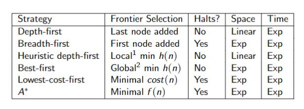
Summary
Adversarial Search
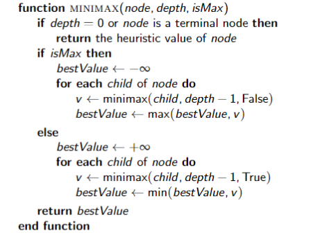
Minimax
For competitive, two-person, zero-sum games
- Try to find the best option for you on nodes that you control (MAX nodes)
- Assumer competitor will take the worst option for you on nodes you do not control (MIN nodes)
- Recursively search to leaf nodes to find the state evaluations, and percolate values upward through the tree
Implementation
Minimax in larger games
Searching all the way to every leaf node is impossibly costly in larger games (e.g. chess)
- Alpha-beta pruning is a method that allows us to ignore portions of the search tree without losing optimality
- It is useful in practical application, but does not change worst-case performance (exponential)
- We can also stop search early by evaluating non-leaf nodes via heuristics
- Can no longer guarantee optimal play
- Can set a fixed maximum depth for the search tree
Higher Level Strategies
The following methods are not full algorithms per se, but can be used to form a strategy for search at a higher level
Direction of Search
The definition of searching is symmetric:
- find path from start nodes to goal node or from goal node to start nodes
Forward branching factor: - Number of arcs out of a node
Backward branching factor: - Number of arcs into a node
Search complexity is, so we should use the direction where the branching factor is smaller
Bidirectional Search
You can search backward from the goal and forward form the start simultaneously
- This wins as
- This can result in an exponential saving in time and space
- The main problem is making sure the frontiers meet
- This is often used with one breadth-first method that builds a set of location that can lead to the goal
- In the other direction another method can be used to find a path to these intersecting locations
Island Driven Search
Idea: find a set of islands between
There are
- This can win as
- The problem is to identify the islands that the path must pass through
- It is difficult to guarantee optimality