Machine Learning

Bayesian Learning

Basic premise:

• have a number of hypotheses or models
• don’t know which one is correct
• Bayesians assume all are correct to a certain degree
• Have a distribution over the models
• Compute expected prediction given this average

Suppose $X$ is input features, and $Y$ is target feature, $d=\{x_1,y_1,x_2,y_2,\cdots ,x_N,y_N\}$ is evidence (data), $x$ is a new input, and we want to know corresponding output $y$.

• We sum over all models, $m\in M$

Bayesian Learning

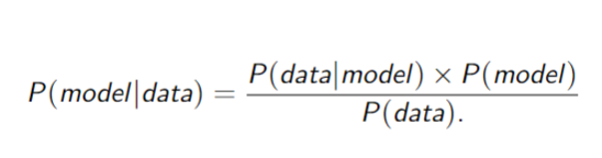
• Prior: $P(H)$
• Likelihood: $P(d|H)$
• Evidence: $d=\{d_1,d_2,\cdots ,d_n\}$
  Bayesian Learning: Update the posterior (Bayes’ Theorem)

Bayesian Prediction

Want to predict $X$: (e.g. next candy)

• Predictions are weighted averages of the predictions of the individual hypotheses
• Hypotheses serve as intermediaries between raw data and prediction

Bayesian Learning Properties

Optimal:

• given prior, no other prediction is correct more often than the Bayesian one
  No overfitting: prior/likelihood booth penalise complex hypotheses

Price to pay:

• Bayesian learning may be intractable when hypothesis space is large
• sum over hypotheses space can be intractable
  Solution: Approximate Bayesian Learning

Maximum a Posteriori

Idea: make a prediction based on most probable hypothesis: $h_{MAP}$

• $h_{MAP}=argma{x}_{h_i}P(h_i|d)$
• $P(X|d)\approx P(X|h_{MAP})$
  Contrast with Bayesian learning where all hypotheses are used

MAP Properties

MAP prediction less accurate than full Bayesian since it relies only on one hypothesis

• MAP and Bayesian predictions converge as data increases
• no overfitting
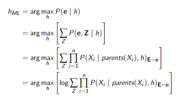
• Finding $h_{MAP}$ may be intractable

* product induces a non-linear optimisation

• can take the log to linearise

Maximum Likelihood (ML)

Idea: Simplify MAP by assuming uniform prior

• i.e. $P(h_i)=P(h_j)\mathrm{\forall }i,j$

Make prediction based on $h_{ML}$ only

ML Properties

ML prediction less accurate than Bayesian or MAP prediction since it ignores prior and relies on one hypothesis

• but ML, MAP and Bayesian converge as the amount of data increases
• more susceptible to overfitting: no prior
• $h_{ML}$ is often easier to find than $h_{MAP}$

Binomial Distribution

Generalise the hypothesis space to a continuous quantity

• $P(Flavour=cherry)=\theta$
• $P(Flavour=lime)=1-\theta$
• $P(klime,ncherry)={\theta }^n(1-\theta {)}^k$ (one order)
• $P(klime,ncherry)=(\genfrac{}{}{0ex}{}{n+k}{k}){\theta }^n(1-\theta {)}^k$ (any order)

Priors on Binomials

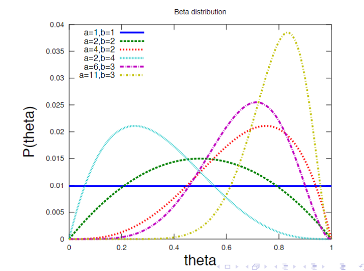
The Beta Distribution $B(\theta ,a,b)={\theta }^{a-1}(1-\theta {)}^{b-1}$

Bayesian Classifiers

Idea: if you knew the classification you could predict the values of features

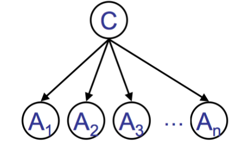
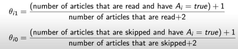
Naïve Bayesian Classifier

$X_i$ are independent of each other given the class

• Requires: $P(Class)$ and $P(X_i|Class)$ for each $X_i$

Predict class $C$ based on attributes $A_i$

• Parameters:
  • $\theta =P(C=true)$
  • ${\theta }_{i1}=P(A_i=true|C=true)$
  • ${\theta }_{i0}=P(A_i=true|C=false)$
• Assumption:
  • $A_i$s are independent given $C$
    
    
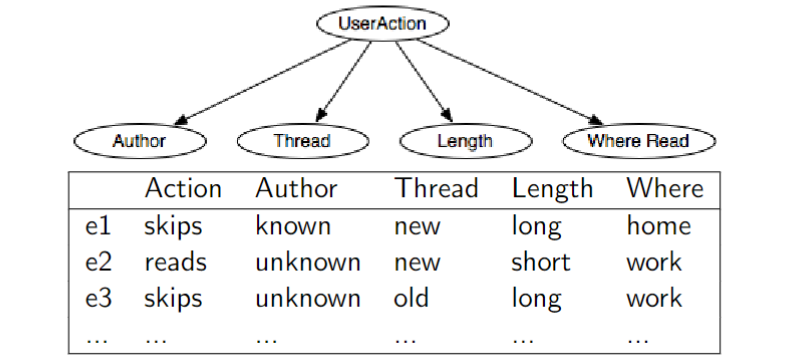
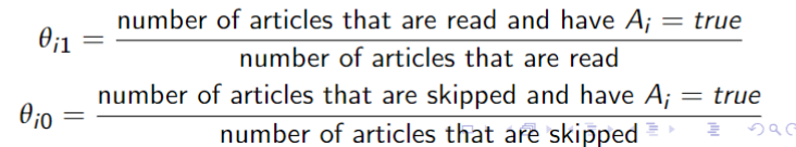
    ML sets:
• $\theta$ to relative frequency of reads, skips
• ${\theta }_{i1}$ to relative frequency of $A_i$ given reads, skips
  

Laplace Correction

If a feature never occurs in the training set, but does in the test set

• ML may assign zero probability to a high likelihood class
• add 1 to the numerator, and add $d$ (arity of variable) to the denominator
• assign:
  • 
• like a pseudocount

Bayesian Network Parameter Learning (ML)

For fully observed data

• Parameters ${\theta }_{V,pa(V)=v^i}$
• CPTS ${\theta }_{V,pa(V)=v}=P(V|Pa(V)=v)$
• Data d:$$d_1 = < V_1=v{1, 1}, V_2 = v_{2, 1},\cdots, V_n=v_{n, 1}>$$$$d_2 = < V_2=v{1, 2}, V_2 = v_{2, 2},\cdots, V_n=v_{n, 2}>$$
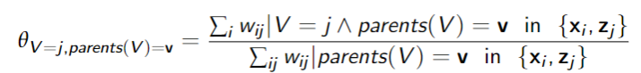
  Maximum likelihood: Set ${\theta }_{V,pa(V)=v}$ to the relative frequency of values of $V$ given the values v of the parents of $V$

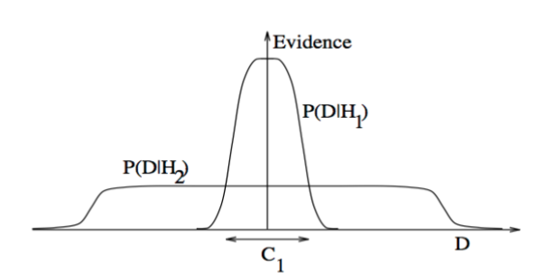
Occam’s Razor

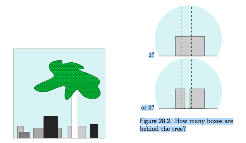
Simplicity is encouraged in the likelihood function:

• $H_2$ is more complex (lower bias) than $H_1$
• so can explain more datasets $D_1$
• but each with lower probability (higher variance)
  

Supervised Machine Learning

Linear Regression

Linear regression is a model in which the output is a linear function of the input features

where $\overrightarrow{w}=<w_0,w_1,w_2,\cdots ,w_n>$. we invent a new feature $X_0\equiv 1$, to make it not a special case.
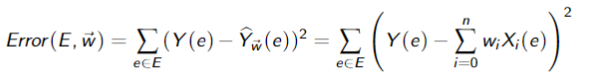
The sum o squares error on examples $E$ for output $Y$ is:$$Error(E, \vec{w}) = \sum_{e\in E}(Y(e)-\hat Y^{\vec w}(e))^2 = \sum_{e\in E}(Y(e)-\sum_{i=0}^nw_iX_i(e))^2$$
Goal: Find weights that minimize $Error(E,\overrightarrow{w})$

Finding weights that minimize $Error$

Find the minimum analytically

• Effective when it can be done
  If
• $\overrightarrow{y}=[Y(e_1),Y(e_2),\cdots ,Y(e_M)]$ is a vector of the output features for the $M$ examples
• $X$ is a matrix where the $j^{th}$ column is the values of the input features for the $j^{th}$ example
• $\overrightarrow{w}=[w_0,w_1,\cdots ,w_n]$ is a vector of weights
  then

$(X{X}^T{)}^{-1}$ is the pseudo-inverse

Find the minimum iteratively

• works for larger classes of problem (not just linear)

Gradient Descent

$\mathrm{\eta }$ is the gradient descent step size, the learning rate
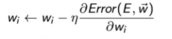
If

then update rule:

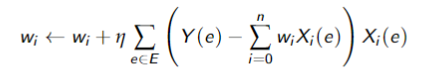
where we have set $\mathrm{\eta }\to 2\mathrm{\eta }$ (arbitrary scale)

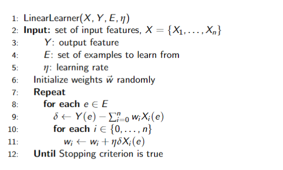
Stochastic and Batched Gradient Descent

• If examples are chosen randomly at line 8 then its stochastic gradient descent
• Batched gradient descent:
  • process a bath of size $n$ before updating the weights
  • if $n$ is all the data, then its gradient descent
  • if $n=1$, its incremental gradient descent
• Incremental can be more efficient than batch, but convergence not guaranteed

Linear Classifier

Assume we are doing binary classification, with classes

• There is no point in making a prediction of less than 0 or greater than 1
• A squashed linear function is of the form:
  
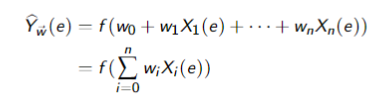
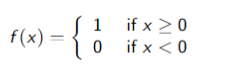
  where $f$ is an activation function
• A simple activation function is the step function:
  

Gradient Descent for Linear Classifiers

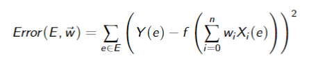
If the activation function is differentiable, we can use gradient descent to update the weights. The sum of squares error:

The partial derivative with respect to weight $w_i$ is:

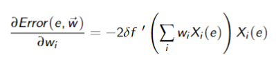
where
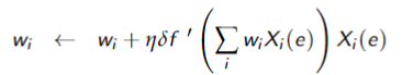
Thus, each example $e$ updates each weight $w_i$ by

The sigmoid or logistic activation function

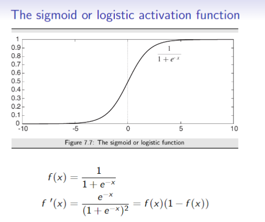
So, $f^{\prime }(x)$ can be computed from $f(x)$

Neural Networks

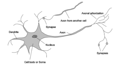
• Inspired by biological networks
• connect up many simple units
• simple neuron: threshold and fire
• can help gain understanding of how biological intelligence works
  
• can learn the same things that a decision tree can
• imposes different learning bias
  • way of making new predictions
• back-propagation learning:
  • errors made are propagated backwards to change the weights
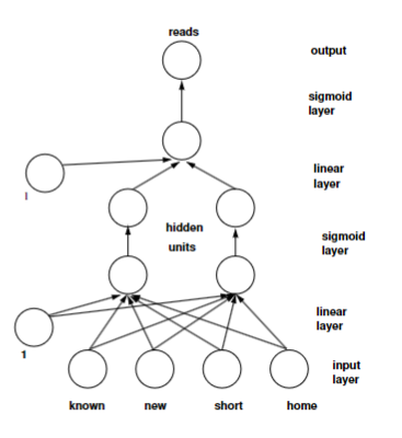
• Often the linear and sigmoid layers are treated as a single layer

Neural Networks Basics

• Each node $j$ has a set of weights $w_{j0},w_{j1},\cdots ,w_{jn}$
• Each node $j$ receives inputs $v_0,v_1,\cdots ,v_N$
• number of weights = number of parents + 1
  • $v_0=1$ constant bias term
• output is the activation function output
  
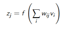
• necessarily non-linear
  • because a linear function of a linear function is a… linear function

Activation Functions

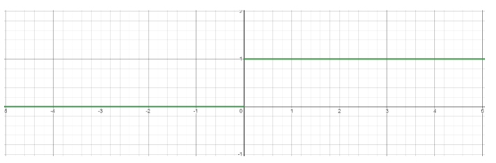
• Step function
  • integrate-and-fire (biological)
  • $f(x)=1$ if $x>0$ else $f(x)=0$
  • simple to use, but not differentiable
  • Not used in practice
    
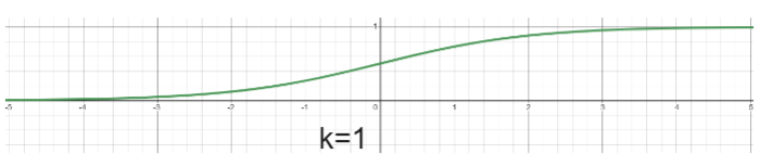
• Sigmoid function
  • $f(x)=\frac{1}{1+e^{0kx}}$
  • For very large or very small $x$, $f(x)$ is very close to 1 or 9
  • Can approximate the step function by tuning $k$
    • As $k$ increases, the sigmoid function becomes steeper and is closer to the step function
    • Usually in practice $k=1$
  • Differentiable
  • Vanishing gradient problem:
    • when $x$ is very large or very small, $f(x)$ responds little to changes in $x$
    • the network does not learn further or learns very slow
  • Computationally expensive
    
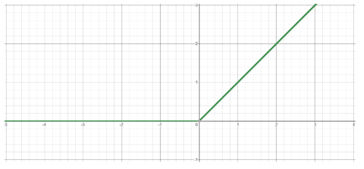
• Rectified Linear Unit (ReLU)
  • $f(x)=max(0,x)$
  • Computationally efficient
    • network converges quickly
  • Differentiable
  • The dying ReLU problem:
    • when inputs approach 0 or are negative, the gradient becomes 0 and the network cannot learn
      
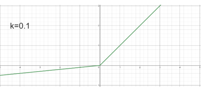
• Leaky ReLU
  • $f(x)=max(0,x)+k\times min(0,x)=max(kx,x)$
  • Small positive slope $k$ in the negative area
    • enables learning for negative input values

Connecting the neurons together in to a network

Feedforward Network

• Forms a directed acyclic graph
• Have connections only in one direction
• Represents a function of its inputs
  Recurrent Network
• Feed its outputs back into its inputs
• Can support short-term memory
  • For the given inputs, the behaviour of the networks depends on its initial state
  • which may depend on previous inputs
• The model is more interesting, but more difficult to understand and to learn

Learning Weights

Back-propagation implements stochastic gradient descent

• Recall:
  
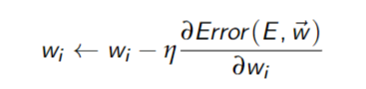
• $\mathrm{\eta }$: learning rate

The Backpropagation Algorithm

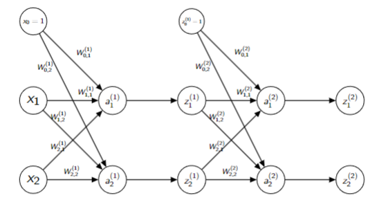
An efficient method of calculating the gradients in a multi-layer neural network

• Given training examples $({\overrightarrow{x}}_n,{\overrightarrow{y}}_n)$ and an error/loss function $Error(\hat{Y},Y)$. Perform 2 passes
  • Forward pass:
    • compute the error $Error$ given the inputs and the weights
  • Backward pass:
    • compute the gradients
• Update each weight by the sum of the partial derivatives for all the training examples

Improving Optimization

• Momentum: weight changes accumulate over iterations
• RMS-Prop: rolling averages of square of gradient
• Adam: combination of Momentum and RMS-Prop
• Initialization: randomly set parameters to start

Improving Generalization: Regularization

Regularized Neural nets: prevent overfitting, increased bias for reduced variance

• parameter norm penalties added to objective function
• dataset augmentation
• early stopping
• dropout
• parameter typing
  • Convolutional neural nets:
    • used for images, parameters tied across space
  • Recurrent neural nets:
    • used for sequences, parameters tied across time

Sequence Modeling

• Word Embeddings:
  • latent vector spaces that represent the meaning of words in context
• RNNs: NN repeats over time and has inputs from previous time step
• LSTM:
  • RNN with longer-term memory
• Attention:
  • uses expected embeddings to focus updates on relevant parts of the network
• Transformers:
  • multiple attention mechanisms
• LLMs:
  • very large transformers for language

Composite models and other learning methods

• Random Forests
  • Each decision tree in the forest is different
    • different features, splitting criteria, training sets
    • average or majority vote determines output
• Support Vector Machines
  • find the classification boundary with the widest margin
  • combine with the kernel trick
• Ensemble Learning
  • combination of base-level algorithms
• Boosting
  • sequence of learners fitting the examples the previous learner did not fit well
    • learners progressively biased towards higher precision
    • early learners:
      • lots of false positives, but reject all the clear negatives
    • later learners:
      • problem is more difficult, but the set of examples is more focused around the challenging boundary

Unsupervised Machine Learning

Incomplete data

Many real-world problems have hidden variables (AKA latent variables)

• incomplete data
• values of some attributes missing
  Incomplete data → unsupervised learning

How to Deal with Missing Data

1. Ignore hidden variables
   • Complexity increases
     
2. Ignore records with missing values
   • does not work with true latent variables
     • e.g. always missing

Often data is missing because of something correlated with a variable of interest

• For example: data in a clinical trial to test a drug may be missing because:
  • the patient dies
  • the patient dropped out because of severe side effects
  • they dropped out because they were better
  • the patient had to visit a sick relative
• ignoring some of these mat make the drug look better or worse than it is
  In general, you need to model why data is missing

3. maximize likelihood directly
   • suppose $Z$ is hidden and $E$ is observable with values $e$
     

Expectation-Maximization (EM)

If we knew the missing values, computing $h_{ML}$ would be easy again!

1. Guess $h_{ML}$
2. iterate:
   • expectation: based on $h_{ML}$, compute expectation of missing values $P(X|h_{ML},e)$
   • maximization: based on expected missing values, compute new estimate of $h_{ML}$

Really simple version (K-means algorithm)

Expectation: based on $h_{ML}$, compute most likely missing values $argma{x}_{Z}P(Z|h_{ML},e)$
Maximization: based on those missing values, you now have complete data

• so compute new estimate of $h_{ML}$ using ML learning as before

K-Means Algorithm

K-means algorithm can be used for clustering:

• dataset of observables with input features $X$ generated by one of a set of classes, $C$
  Inputs:
• training examples
• the number of classes, $k$
  Outputs:
• a representative value for each input feature for each class
• an assignment of examples to classes
  Algorithms:

1. pick $k$ means in $X$, one per class, $C$
2. iterate until means stop changing:
   1. assign examples to $k$ classes (e.g. as closest to current means)
   2. re-estimate $k$-means based on assignment

Expectation Maximization

Approximate the maximum likelihood

• Start with a guess $h_0$
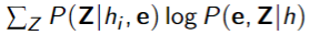
• Iteratively compute:
  
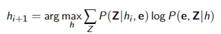
• expectation: compute $P(Z|h_i,e)$
  • ”fills in” missing data
• maximization: find new $h$ that maximizes
  
• can show that $P(e|h_{i+1}))\ge P(e|h_i)$ when computed like this

General Bayes Network EM

Complete Data: Bayes Net Maximum Likelihood

$parents(V)$: parents of $V$
Incomplete data: Bayes Net Expectation Maximization

• observed variables $X$ and missing variables $Z$
• Start with some guess for $\theta$
  E Step: Compute weights for each data $x_i$ and latent variable(s) value(s) $z_j$
• using e.g. variable elimination
  
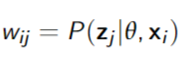
  M Step: Update parameters:
  

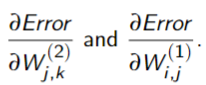
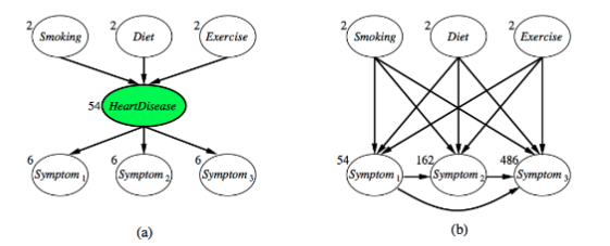
Belief Network Structure Learning

• A model here is a belief network
• A bigger network can always fit the data better
• $P(model)$ lets us encode a preference for smaller networks
  • e.g. using the description length
• You can search over network structure looking for the most likely model
  Can do independence tests to determine which features should be the parents
• XOR problem:
  • just because features do not give information individually, does not mean they will not give information in combination
• ideal: Search over total orderings of variables

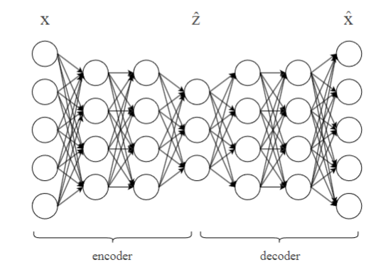
Autoencoders

A representational learning algorithm

• Learn to map examples to low-dimensional representation

Components

2 main components:

1. Encoder $e(x)$: maps $x$ to low-dimensional representation $\hat{z}$
2. Decoder $d(\hat{z})$: maps $\hat{z}$ to its original representation $x$
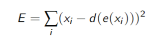
   Autoencoder implements $\hat{x}=d(e(x))$

• $\hat{x}$ is the reconstruction of original input $x$
• Encoder and decoder learned such that $\hat{z}$ contains as much information about $x$ as needed to reconstruct it
  Minimize sum of squares of differences between input and prediction:
  

Deep Neural Network Autoencoders

• good for complex inputs
• $e$ and $d$ are feedforward neural networks, joined in series
• Train with backpropagation
  

Generative Adversarial Networks

A generative unsupervised learning algorithm

• Goal is to generate unseen examples that look like training examples
  

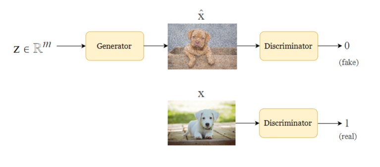
Components

GANs are actually a pair of neural networks:

• Generator $g(z)$: Given vector $z$ in latent space, produces example $x$ drawn from a distribution that approximates the true distribution of training examples
  • $z$ sampled from a Gaussian distribution
• Discriminator $d(x)$: A classifier that predicts whether $x$ is real (from training set) or fake (made by $g$)

Training

GANs are trained with a minimax error:

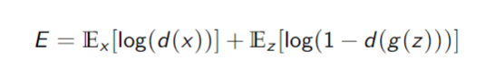
• Discriminator tries to maximize $E$
  • for $x$ from the training set, $d(x)\to 1$
  • for $x$ from the generator, $d(x)\to 0$
• Generator tries to minimize $E$ - tries to fool $d$
  • for $x$ from the training set, $d(x)\to 0$
  • for $x$ from the generator, $d(x)\to 1$
    After convergence:
• $g$ should be producing realistic images
• $d$ should output $\frac{1}{2}$, indicating maximal uncertainty