Ordinary Differential Equations

General for of an ODE

F (n, y (n), y^{(1)} (n), y^{(2)} (n), \dots, y^{(n)} (n)) = 0

where $y^{(i)} (n)$ is the $i^{t h}$ derivative of $y (n)$

The highest order of the derivatives is called the order of the ordinary differential equation.

A closed-form is often unavailable in practice!

Instead we may know a relationship between variable $y$ and its derivative $y^{'}$ given by a known function $f$ :

y^{'} (t) = f (t, y (t))

The speed

v (t)

of a car changes based on forces applied to it:

$v^{'} (t) = F (t) / m$

Initial Value Problem

The general form is a differential equation

y^{'} (t) = f (t, y (t))

where $f$ is specified, and the initial values are

y (t_{0}) = y_{0}

There are two ways that out ODE problems will become more complicated

By involving more than one unknown variable (not just $y$ ): Systems of differential equations
By solving second, third, or higher derivatives (not just $y^{'}$ ): Higher order differential equations

Systems of Differential Equations

Consider a model with multiple variables that interact:

E.g. $x$ and $y$ coordinates of a moving object.
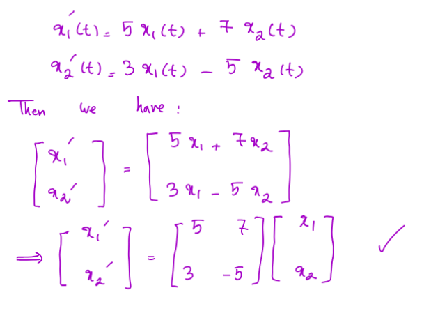
This gives a system of differential equations, such as
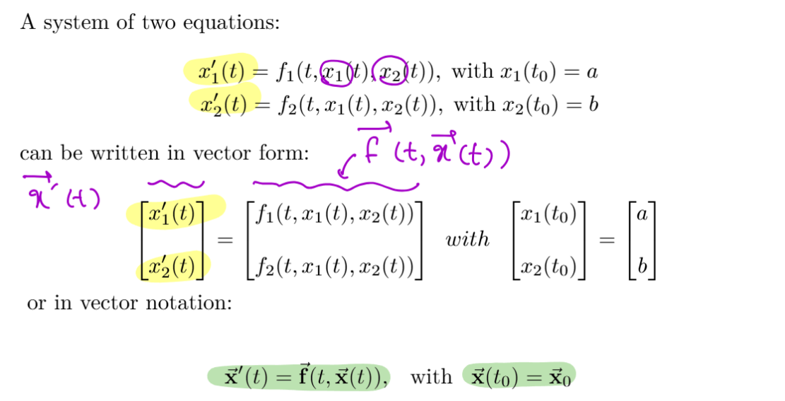
The matrix notation is specially helpful when $f_{1}$ and $f_{2}$ are linear
- The $\vec{f}$ can be decomposed as a constant matrix and a vector containing the functions

Example

Pasted image 20250303093328.png

Higher Order Differential Equations

To start, we consider 1st order ODEs, involving only first derivative

y^{'} (t) = f (t, y (t)) $ $ H i g h e r d e r i v a t i v e s o c c u r o f t e n i n r e a l p r o b l e m s . T h e o r d e r i s t h e h i g h e s t d e r i v a t i v e i n t h e e q u a t i o n : $ $ y^{(n)} (t) = f (t, y (t), y^{'} (t), y^{″} (t), y^{‴} (t), \dots, y^{(n - 1)} (t))

Numerical Schemes for ODEs

Numerical solution is a discrete set of time/value pairs, $(t_{i}, y_{i})$

What will an approximate solution look like?

$y_{i}$ should approximate the true value, $y (t_{i})$

Time-Stepping

Given initial conditions, we repeatedly step sequentially forward to the next time instant, using the derivative info, $y^{'}$ , and a timestep, h.
Set $n = 0, t = t_{0}, y = y_{0}$ :

Compute $y_{n + 1}$
Increment time, $t_{n + 1} = t_{n} + h$
Advance, $n = n + 1$
Repeat

Categorizing time-stepping methods

Single-step vs Multistep:

Do we use information only from he current time or from previous timesteps too?
Explicit vs Implicit:
Is $y_{n + 1}$ given as an explicit function to evaluate, or do we need to solve an implicit equation?
Timestep size:
Do we use a constant timestep $h$ , or allow it to vary?

Trade-offs

Explicit:

Simpler and fast to compute per step
Less stable - require smaller timesteps to avoid “blowing up”
Implicit:
Often more complex and expensive to solve per step
More stable - can safely use larger timesteps

Time-Stepping as a Recurrence

Time-stepping applies a recurrence relation to approximate the function values at later and later times

Given $y_{0}$ , approximate $y_{1}$ . Given $y_{1}$ , approximate $y_{2}$ . etc.

Time-Stepping as a “Time Integration”

Time-stepping is also known as “time-integration”:

We are integrating over time to approximate $y$ from $y^{'}$
- Approximating area under the curve
  Better time-stepping schemes correspond to better approximations of the integral

Error of Time-Stepping

Absolute / global error at step $n$ is $| y_{n} - y (t_{n}) |$

We can’t measure error exactly without knowing $y (t)$
We will rely on the Taylor series

Forward Euler

Explicit, single-step scheme

Compute the current slope: $y_{n}^{'} = f (t_{n}, y_{n})$
Step in a straight line with that slope: $y_{n + 1} = y_{n} + h \cdot y_{n}^{'}$

y_{n + 1} = y_{n} + h f (t_{n}, y_{n})

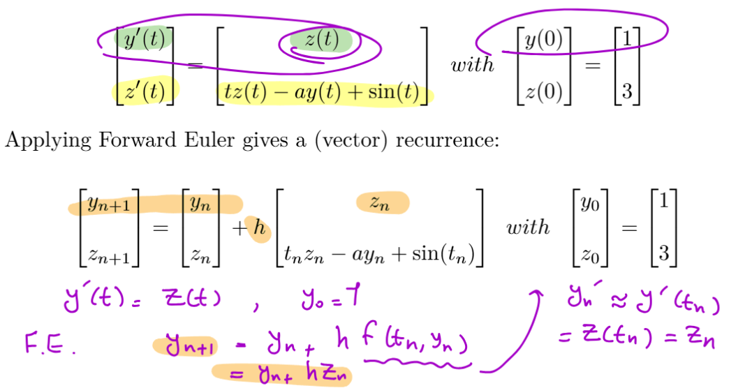
System of Equations

For systems of 1st order ODEs, we apply Forward Euler to each row in exactly the same way.

Example

Pasted image 20250303101510.png

Error of Forward Euler Method

F.E. is $$y_{n+1} = y_n + hf(t_n, y_n)$$
Taylor series is:

y_{(} t_{n + 1}) = y (t_{n}) + h y^{'} (t_{n}) + \frac{h^{2}}{2!} y^{″} (t_{n}) + \frac{h^{3}}{3!} y^{‴} (t_{n}) + \dots

The error for one step is the difference between these, assuming exact data at time $t_{n}$

i.e. $y_{n} = y (t_{n})$
In this case, Forward Euler becomes:

y_{n + 1} = y (t_{n}) + h y^{'} (t_{n})

The difference is:

y_{n + 1} - y (t_{n + 1}) = - \frac{h^{2}}{2!} y^{″} (t_{n}) + O (h^{3}) = O (h^{2})

This is the Local Truncation Error (LTE) of Forward Euler!

As $h$ decreases, LTE decreases quadratically

More accurate time-stepping

Keeping more terms in the series will help derive higher order schemes!

We don’t know

y^{″}

Use a finite difference to approximate

y^{″}

$y^{″} (t_{n}) = \frac{y^{'} (t_{n + 1}) - y^{'} (t_{n})}{h} + O (h)$

Trapezoidal Rule

Trapezoidal Scheme is:

y_{n + 1} = y_{n} + \frac{h}{2} [f (t_{n + 1}, y_{n + 1}) + f (t_{n}, t_{n})]

The Local Truncation Error for trapezoidal rules is $O (h^{3})$

Called trapezoidal because it turns the rectangles in integration into trapezoids

Pasted image 20250303103700.png

This is an implicit scheme

Can we make it explicit?

Modified / Improved Euler

Take forward Euler step to estimate the end point
Evaluate slope there
Use this approximate end-of-step slope in the trapezoidal formula
This looks like:

$y_{n + 1}^{*} = y_{n} + h f (t_{n}, y_{n})$
$y_{n + 1} = y_{n} + \frac{h}{2} (f (t_{n}, y_{n}) + f (t_{n + 1}, y_{n + 1}^{*}))$
Explicit scheme with LTE $O (h^{3})$

Backwards Euler Method

Implicit Scheme

Similar to forward Euler

y_{n + 1} = y_{n} + h f (t_{n + 1}, y_{n + 1})

Its LTE is $O (h^{2})$ , like forward Euler

Explicit “Runge Kutta” schemes

Pasted image 20250303111155.png
A family of explicit schemes (including improved Euler) written as:
$k_{1} = h f (t_{n}, y_{n})$
$k_{2} = h f (t_{n} + h, y_{n} + k 1)$
$y_{n + 1} = y_{n} + \frac{k_{1}}{2} + \frac{k_{2}}{2}$

4th Order Runge Kutta

LTE of $O (h^{5})$
Similar schemes exist for higher orders, $O (h^{α})$ for $α = 3, 4, 5, 6, \dots$
$k_{1} = h f (t_{n}, y_{n})$
$k_{2} = h f (t_{n} + \frac{h}{2}, y_{n} + \frac{k_{1}}{2})$
$k_{3} = h f (t_{n} + \frac{h}{2}, y_{n} + \frac{k_{2}}{2})$
$k_{4} = h f (t_{n} + h, y_{n} + k 3)$
$y_{n + 1} = y_{n} + \frac{1}{6} (k_{1} + 2 k_{2} + 2 k_{3} + k_{4})$
Again, evaluate $y^{'} (t) = f (t, y)$ at various intermediate positions, and take a specific combination to find $y_{n + 1}$

Midpoint Method

Another explicit Runge Kutta scheme with LTE $O (h^{3})$
$k_{1} = h f (t_{n}, y_{n})$
$k_{2} = h f (t_{n} + \frac{h}{2}, y_{n} + \frac{k 1}{2})$
$y_{n + 1} = y_{n} + k_{2}$
Equivalent Expression
$y_{n + \frac{1}{2}}^{*} = y_{n} + \frac{h}{2} f (t_{n}, y_{n})$
$y_{n + 1} = y_{n} + h f (t_{n} + \frac{h}{2}, y_{n + \frac{1}{2}}^{*})$

Local vs Global Error

The Global Error is the total error accumulated at the final time $t_{f i n a l}$

Global error is typically more important since our goal is to predict some final future value
For a constant step $h$ , computing from $t_{0}$ to end time $t_{f i n a l}$

# s t e p s = \frac{t_{f i n a l} - t_{0}}{h} = O (h^{- 1})

Then, for a given method we have:

(Global Error) \leq (Local Error) \cdot O (h^{- 1})

i.e. one degree lower than LTE

Multi-step Schemes

One way to derive them is by fitting curves to current and earlier data points, for better slope estimates.
E.g. fit a quadratic to previous, current, and next step

Backward Differentiation Formulas Methods (BDF)

BDF1, BDF2, BDF3, etc.

Number indicates order of global error
BDF1 = Backward Eular
Generalize the backwards Euler scheme

y_{n + 1} = y_{n} + h f (t_{n + 1}, y_{n + 1})

to higher order using earlier step info.

BDF2 uses current and previous step data:

y_{n + 1} = \frac{4}{3} y_{n} - \frac{1}{3} y_{n - 1} + \frac{2}{3} h f (t_{n + 1}, y_{n + 1})

BDF has LTE $O (h^{3})$ and is a multi-step scheme

General Form

The same approach extends to higher orders, yielding implicit schemes with the general form

\sum_{k = - s + 1}^{1} a_{k} y_{n + k} = h f (t_{n + 1}, y_{n + 1})

With $a_{k}$ being the coefficients.

Explicit Multistep Scheme

Adams-Bashforth

e.g. 2nd order:

y_{n + 1} = y_{n} + \frac{3}{2} h f (t_{n}, y_{n}) - \frac{1}{2} h f (t_{n - 1}, y_{n - 1})

LTE is $O (h^{3})$

Higher Order ODEs

The order of the ODE is the highest derivative that appears

e.g. an ODE with at most third derivates gives a 3rd order ODE

Converting to First Order

The general form for such a higher ODE looks like

y^{(n)} = f (t, y (t), y^{(1)} (t), y^{(2)} (t), \dots, y^{(n - 1)} (t))

We can convert them to systems of first order ODEs

Change of variables
For each variable $y$ with more than a first derivative, introduce new variables:

y_{i} = y^{(i - 1)}

for $i = 1$ to $n$ , so each derivative has a corresponding new variable
Substituting the new variables into the original ODE leads to:

One first order equation for each original equation
One or more additional equations relating the new variables

Stability of Time-Stepping Schemes

Since errors are generally $O (h^{p})$ for some $p$ , our schemes are less accurate for large $h$ .

But, error/perturbations in initial conditions may lead to vastly different or incorrect answers.

y^{'} (t) = f (t, y (t)), y (0) = y_{0} + ϵ_{0}

If some initial error $ϵ_{0}$ grows exponentially for many steps, our time-stepping scheme is unstable.

Test Equation

We’ll consider a simple linear ODE, our “test equation”,

y^{'} (t) = - λ y (t), y (0) = y_{0}

for constant $λ > 0$ .
The exact solution is $y (t) = y_{0} e^{- λ t}$

Tends to 0 as $t \to \infty$

Our Approach

Apply a given time stepping scheme to our test equation
Find the closed form of its numerical solution and error behaviour
Find the conditions on the timestep $h$ that ensure stability (error approaching zero)

Stability of Forward Euler

It is conditionally stable when $0 < h < \frac{2}{λ}$

Stability of Backward/Implicit Euler

It is unconditionally stable

Stability does not imply accuracy!

Large time steps still usually induce Large truncation error

Stability of Improved Euler

It is conditionally stable when $h < \frac{2}{λ}$

Same as Forward Euler

Stability in general

For our linear test equation $y^{'} = - λ y$ , forward Euler gave a bound related to

λ = | \frac{\partial}{\partial y} (λ y) = | \frac{\partial f}{\partial y} |

For nonlinear problems, stability depends on $\frac{\partial f}{\partial y}$ (for dynamics function $f$ ) evaluated at a given point in time/space
For systems of ODEs, stability relates to the eigenvalues of the “Jacobian” matrix

\frac{\partial (f_{1}, f_{2}, f_{3}, \dots, f_{n})}{\partial (y_{1}, y_{2}, y_{3}, \dots, y_{n})}

Truncation Error vs Stability

Stability tells us what our numerical algorithm itself does to small errors
Truncation error tells us how the accuracy of our numerical solution scales with time step $h$

Both factors should be considered to get a useful solution

Determining LTE

Replace approximations on RHS with exact versions
Taylor expand all RHS quantities about time $t_{n}$
Taylor expand the exact solution $y (T_{n + 1})$ to compare against
Compute difference $y (t_{n + 1}) - y_{n + 1}$ . Lowest degree non-cancelling power of $h$ gives the LTE

Time Step Control

Trade-offs

Smaller $h$ : many steps, computationally expensive, more accurate
Larger $h$ : fewer steps, so cheaper, but also less accurate
Minimize effort/cost by choosing largest $h$ with error still less than a desired tolerance:

error < tolerance

Adaptive Time-Stepping

Rate of change of the solution often varies over time!

Adapt the time step during the computation to keep error small, while minimizing wasted effort

Problem

If we knew the error for a given $h$ , we could choose a good $h$ to always satisfy error < tolerance

… but if we already knew the exact error, we’d also know the solution

Approach

Use two different time-stepping schemes together. Compare their results to estimate the error, and adjust $h$ accordingly

Adaptive Time-Stepping using Order $p$ and Order $p + 1$ methods

Idea:

Run 2 methods simultaneously with different truncation error orders
Approximate the error as $e r r = | y_{n + 1}^{A} - y_{n + 1}^{B} |$ where $y_{n + 1}^{A}$ has $O (h^{p})$ and $y_{n + 1}^{B}$ has $O (h^{p + 1})$
If err > threshold, reduce $h$ (halve it) and recompute the step again, until the threshold is satisfied
Estimate the error coefficient $c$ as

c \approx \frac{| y_{n + 1}^{A} - y_{n + 1}^{B} |}{h_{o l d}^{p}}

where $h_{o} l d$ is the most recent time step size. If $c$ changes slowly in time, we can estimate the next step error as:

e r r_{n e x t} = | y_{n + 2}^{A} - y (t_{n + 2}) | \approx c (h_{n e w})^{p}

plug in $c$ :

e r r_{n e x t} \approx \frac{| y_{n + 1}^{A} - y_{n + 1}^{B} |}{h_{o l d}^{p}} (h_{n e w})^{p} = (\frac{h_{n e w}}{h_{o l d}})^{p} | y_{n + 1}^{A} - y_{n + 1}^{B} |

Given a desired error tolerance $t o l$ , set $e r r_{n e x t} = t o l$ and solve for $h_{n e w}$ :

h_{n e w} = h_{o l d} (\frac{t o l}{| y_{n + 1}^{A} - y_{n + 1}^{B} |})^{1 / p}

To (roughly) compensate for our approximations, we may be conservative by scaling $t o l$ down by some factor $α$ , e.g. $α = 1 / 2$ , or $α = 3 / 4$ . This will allow step size to grow larger again when it is likely safe to do so.

Ordinary Differential Equations

General for of an ODE

Initial Value Problem

Systems of Differential Equations

Higher Order Differential Equations

Numerical Schemes for ODEs

Time-Stepping

Categorizing time-stepping methods

Trade-offs

Time-Stepping as a Recurrence

Time-Stepping as a “Time Integration”

Error of Time-Stepping

Forward Euler

System of Equations

Error of Forward Euler Method

More accurate time-stepping

Trapezoidal Rule

Modified / Improved Euler

Backwards Euler Method

Explicit “Runge Kutta” schemes

4th Order Runge Kutta

Midpoint Method

Local vs Global Error

Multi-step Schemes

Backward Differentiation Formulas Methods (BDF)

BDF2 uses current and previous step data:

General Form

Explicit Multistep Scheme

Adams-Bashforth

Higher Order ODEs

Converting to First Order

Stability of Time-Stepping Schemes

Test Equation

Our Approach

Stability of Forward Euler

Stability of Backward/Implicit Euler

Stability of Improved Euler

Stability in general

Truncation Error vs Stability

Determining LTE

Time Step Control

Trade-offs

Adaptive Time-Stepping

Approach

Adaptive Time-Stepping using Order p and Order p+1 methods

Adaptive Time-Stepping using Order $p$ and Order $p + 1$ methods