Numerical Linear Algebra

The study of algorithms for performing linear algebra operations numerically

• Matrix/vector arithmetic
• Solving linear systems of equations
• Taking norms
• Factoring & inverting systems of equations
• Finding eigenvalues/eigenvectors
  Numerical methods often differ from familiar exact methods, due to:
• efficiency concerns
• floating point error
• stability
• etc.

Page Rank

Idea: If many web pages link to your website, there must be a consensus that it is important

Web Links as a Graph

We represent the web’s structure as a directed graph

• Nodes (circles) represent pages
• Arcs (arrows) represent links from one page to another
  We will use degree to refer to a node’s outdegree
• the number of arcs leaving the node

Adjacency Matrix

Then the degree for node $q$ is the sum of entries in column $q$
Notice: Matrix $G$ is not necessarily symmetric about the diagonal

Interpreting Links as Votes

If page $j$ links to page $i$, this is considered a vote by $j$ that $i$ is important

• Outgoing links of a page $j$ have equal influence, so the importance that $j$ gives to $i$ is: $$\frac{1}{deg(j)}$$

Global Importance

If page $i$ has many incoming links, it is probably important

• What if page $i$ has just one incoming link, but the link is from page $j$, and $j$ has many incoming links?
  • Then $i$ is probably fairly important too!

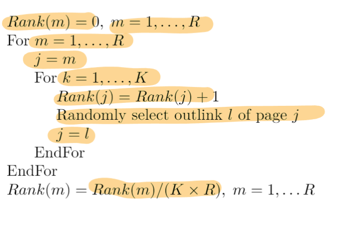
The Random Surfer Model

Imagine an internet user who starts at a page, and follows links at random from page to page for K steps

• They will probably end up on important pages more often
  Then, select a new start page, and follow $K$ random links again. Repeat the process $R$ times, starting from each page.
  At the end, we estimate overall importance as:$$\text{Rank(page i) = (Visits to page i)/(Total visits to all pages) = (Visits to page i)/($R\times K$)}$$

Criticisms

Potential issues with this algorithm?

• The number of real web pages is monstrously huge
  • ~1 billion unique hostnames
  • many iterations needed
• Number of steps is taken per random surf sequence must be large, to get a representative sample
• What about dead end links?
  • stuck on one page!
• What about cycles in the graph?
  • Stuck on a closed subset of pages

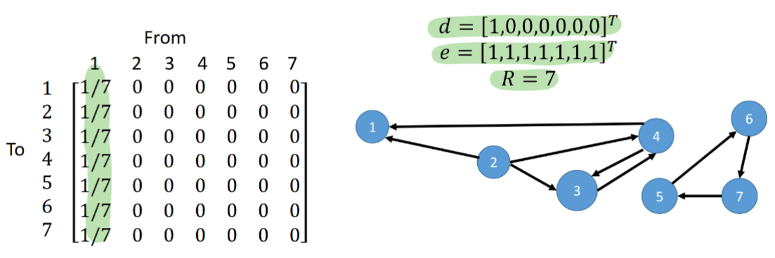
A Markov Chain Matrix

Let $P$ be a (large!) matrix of probabilities, where $P_{ij}$ is the probability of randomly transitioning from page $j$ to page $i$

We can build this matrix $P$ from our adjacency matrix $G$

• Divide all entries of each column of $G$ by the column sum (out-degree of the node)

Dead Ends

To deal with dead-end links, we will simply teleport to a new page at random!

• if $R$ is the number of pages, we augment $P$ to get $P^{\prime }$ defined by:$$P' = P+\frac{1}{R}ed^T$$
• The matrix $\frac{1}{R}e{d}^T$ is a matrix of probabilities such that from any dead end page $(d_i=1)$, we transition to every other page with equal probability
  

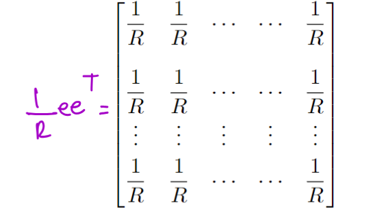
Escaping Cycles

Most of the time (a fraction $\alpha$), follow links randomly, via $P^{\prime }$

• Occasionally wish some probability, $(1-\alpha )$, teleport from any page to any other page with equal probability, regardless of links$$M=\alpha P'+(1-\alpha)\frac{1}{R}ee^T$$
• The $\frac{1}{R}e{e}^T$ matrix looks like:
  
  We will call the combined matrix $M=\alpha P^{\prime }+(1-\alpha )\frac{1}{R}e{e}^T$ our Google matrix
• Most of the time this just follows links
  • and always teleports out of dead ends
• Also occasionally teleports randomly to escape cycles
  Google purportedly used $\alpha \approx 0.85$
  The sum of each column is 1

Some Useful Properties of $M$

The entries of $M$ satisfy $0\le M_{ij}\le 1$
Each column of $M$ sums to 1$$\sum_{i=1}^RM_{ij} = 1$$
Interpretation: If we are on a webpage, probability of being on some webpage after a transition is 1

• we can’t just disappear

Markov Transition Matrices

The Google Matrix $M$ is an example of a Markov matrix
We define a Markov matrix $Q$ by the two properties:

Probability Vector

Now, define a probability vector as a vector $q$ such that

If the surfer starts at a random page with equal probabilities, this can be represented by a probability vector, where $p_i=\frac{1}{R}$

• If a surfer starts at a specific page, that entry will have probability 1 and others will have probability 0

Evolving the Probability Vector

Now we have:

• the probability vector describing the initial state, $p^0$
• a Markov matrix $M$ describing the transition probabilities among pages
  Their product $M{p}^0$ tells us the probabilities of our surfer being at each page after one transition

Preserving a Probability Vector

If $p^n$ is a probability vector, is $p^{n+1}=M{p}^n$ also a probability vector?

• Yes!

Page Rank Idea

With what probability does our surfer end up at each page after many steps, starting from $p^0=\frac{1}{R}e$?

• i.e. What is $p^{\mathrm{\infty }}=\underset{k\to \mathrm{\infty }}{lim}(M{)}^k{p}^0$?
• higher probability in $p^{\mathrm{\infty }}$ implies greater importance
  • then we can rank the pages by this importance measure
    Questions:
• Do we actually know if it will settle/converge to a fixed final result
• If yes, then how long will it take? Roughly how many iterations are needed before we can stop?
• Can we implement this efficiently?

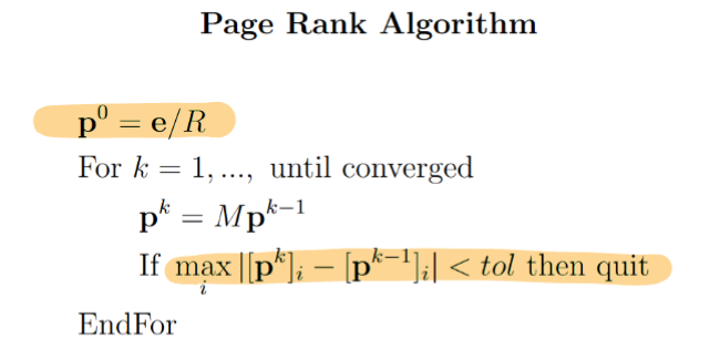
Making Page Rank Efficient

How can we apply/implement Page Rank in a way that is computationally feasible?

• We’ll exploit precomputation and sparsity

Precomputation

The ranking vector $p^{\mathrm{\infty }}$ can be precomputed once and stored, independent of any specific query

• to later search for a keyword, Google finds only the subset of pages matching the keywords, and ranks those by their precomputed values in $p^{\mathrm{\infty }}$

Sparsity

In numerical linear algebra, we often deal with two kinds of matrices

• Dense: Most or all entries are non-zero. Store in an $N\times N$ array, manipulate “normally”
• Sparse: Most entries are zero. Use a “sparse” data structure to save space and time
  • prefer algorithms that avoid “destroying” sparsity

Sparse Matrix-Vector Multiplication

Multiplying a sparse matrix with a vector can be done efficiently

• Only non-zero matrix entries are ever accessed/used
  

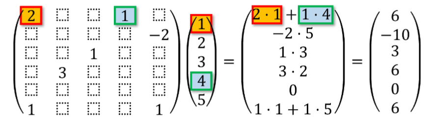
Exploiting Sparsity

Note: $M$ is fully dense to escape cycles
The trick: Use linear algebra manipulations to perform the main iteration$$p^{n+1}=Mp^n$$without ever creating/storing $M$!
Recall:

Consider computing:

We never form $M$ explicitly

Google Search: Other Factors

Page Rank can be “tweaked” to incorporate other (commercial?) factors.

Replace standard teleportation $(1-\alpha )\frac{1}{R}e{e}^T$ with $(1-\alpha )v{e}^T$, where a special probability vector $v$ places extra weight on whatever sites you like.

• In modern search engines, many factors beside pure link-based ranking can come into play

Convergence of Page Rank

We will need some additional facts about Markov Matrices, involving eigenvalues and eigenvectors

Eigenvalues and Eigenvectors

An eigenvalue $\lambda$ and corresponding eigenvector $x$ of a matrix $Q$ are a scalar and non-zero vector, respectively, which satisfy$$Qx=\lambda x$$
Equivalently, this can be written as$$Qx=\lambda I x$$where $I$ is the identity matrix
Rearranging gives$$(\lambda I - Q)x = 0$$which implies that the matrix $\lambda I-Q$ must be singular for $\lambda$ and $x$ to be an eigenvalue/eigenvector pair, since we want $x\ne 0$

Singular

A singular matrix $A$ satisfies $detA=0$
Thus to find the eigenvalues $\lambda$ of $Q$, we can solve the characteristic polynomial given by $$\det(\lambda I -Q) = 0$$which is $$(\lambda - Q_{00})(\lambda-Q_{11})-(Q_{01}\times Q_{10})=0$$solve for $\lambda$
plug $\lambda$ back in $Qn=\lambda n$ to find corresponding eigenvectors

Properties

det(A − λI) = 0 → eigenvalues

• tr(A) = sum of eigenvalues
• det(A) = product of eigenvalues
• A invertible ⇔ 0 not an eigenvalue
• A diagonalizable ⇔ n lin. indep. eigenvectors
• Symmetric ⇒ diagonalizable w/ real eigenvalues
• Triangular ⇒ eigenvalues = diagonal entries

Convergence Properties

1. Every Markov matrix $Q$ has 1 as an eigenvalue
2. Every eigenvalue of a Markov matrix Q satisfies $|\lambda |\le 1$
   1. So 1 is the largest eigenvalue
3. A Markov matrix $Q$ is a positive Markov matrix if $Q_{ij}>0\mathrm{\forall }i,j$
4. If $Q$ is a positive Markov matrix, then there is only one linearly independent eigenvector of $Q$ with $|\lambda |=1$
   The number of iterations required for Page Rank to converge to the final vector $p^{\mathrm{\infty }}$ depends on the size of the 2nd largest eigenvalue, $|\lambda 2|$

• Then 2nd largest eigenvalue dictates the slowest rate at which the unwanted component of $p^0$ are shrinking

Result

For google matrix, $|\lambda |\approx alpha$

• where $\alpha$ dictated the balance between following real links, and teleporting randomly

A smaller value of $|{\lambda }_2|\approx \alpha$ implies faster convergence

• Should we speed it up by choosing a small $\alpha$?
  NO! $\alpha =0$ implies only random teleportation.
• $\alpha$ trades off accuracy for efficiency

Gaussian Elimination

Solving Linear Systems of Equations

Cost of Triangular Solve

Triangular solves cost $n^2+O(n)$ FLOPs each, so total is $2n^2+O(n)$
Factorization cost dominates when $n$ is large, and scales worse

• Given an existing factorization, solving for new RHS’s is cheap: $O(n^2)$

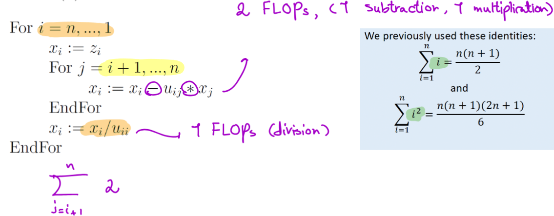
Row Subtraction via Matrices

Zeroing a (sub-diagonal) entry of a column by row subtraction can be written as applying a specific matrix $M$ such that

where

• $A^{old}$ is the original matrix
• $A^{new}$ is the matrix after subtracting the specific row

can be written as a matrix:

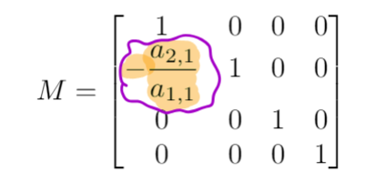
• $M$ is the identity matrix, but with a zero entry replaced by the (negative of the) necessary multiplicative factor
  So, the whole process of factorization can be viewed as a sequence of matrix (left-)multiplications applied to $A$
• The matrix left at the end is $U$

Therefore:

• Define $L=(M^{(1)}{)}^{-1}(M^{(2)}{)}^{-1}(M^{(3)}{)}^{-1}$ and we have our factorization!
  Interleaving the permutation matrices $P^{(k)}$ before each $M^{(k)}$ similarly leads to the $PA=LU$ factorization

Inverse of $M^{(i)}$

What is $(M^{(k)}{)}^{-1}$?

• The inverse of the simple matrix form is the same matrix, but with the off–diagonal entry negated

Costs: Solving $Ax=b$ by Matrix Inversion

An obvious alternative for solving $Ax=b$ is:

1. Inver $A$ to get $A^{-1}$
2. Multiply $A^{-1}b$ to get $x$
   One can show that the above is actually more expensive than using our factor and triangular solve strategy

• It also generally incurs more floating point error
• Most numerical algorithms avoid ever computing $A^{-1}$

Norms and Conditioning

Norms are measurements of “size”/magnitude for vectors or matrices
Conditioning describes how the output of a function/operation/matrix changes due to changes in input

Vector Norms

There are many reasonable norms for a vector, $x=[x_1,x_2,\cdots ,x_n{]}^T$
Common choices are:

1. 1-norm (or taxicab/Manhattan norm): $\parallel x{\parallel }_1=\sum _{i=1}^n|x_i|$
2. 2-norm (or Euclidean norm): $\parallel x{\parallel }_2=\sqrt{\sum _{i=1}^n{x}_i^2}$
3. $\mathrm{\infty }$-norm (or max norm): $\parallel x{\parallel }_{\mathrm{\infty }}=\underset{i}{max}|x_i|$

$p$-norms

These are collectively called $p$-norms, for $p=1,2,\mathrm{\infty }$ and can be written: $$|x|p=\left(\sum^n|x_i|^p\right)^\frac{1}{p}$$

• Only holds in the limit for $\mathrm{\infty }$ case

Key Properties of Norms

If the norm is zero, then the vector must be the zero-vector

The norm of a scaled vector must satisfy

The triangle inequality holds:

Defining Norms for Matrices

Matrix norms are often defined/”induced” as follows, using $p$-norms of vectors:

• Clearly we can’t try out all possible $x$ to determine this
• There are simpler equivalent definitions in some cases:
  • Max absolute column sum

* Max absolute row sum

Matrix 2-norm

Using the vector 2-norm, we get the matrix 2-norm, or spectral norm:

The matrix’s 2-norm relates to the eigenvalues
Specifically, if ${\lambda }_i$ are the eigenvalues of $A^{T}A$, then

Matrix Norm Properties

1. $\parallel A\parallel =0⟺A_{ij}=0\mathrm{\forall }i,j$
2. $\parallel \alpha A\parallel =|\alpha |\cdot \parallel A\parallel$ for all scalar $\alpha$
3. $\parallel A+B\parallel \le \parallel A\parallel +\parallel B\parallel$
4. $\parallel Ax\parallel \le \parallel A\parallel \cdot \parallel x\parallel$
5. $\parallel AB\parallel \le \parallel A\parallel \cdot \parallel B\parallel$
6. $\parallel I\parallel =1$

Conditioning of Linear Systems

Conditioning describes how the output of a function/operation/problem changes due to changes in input

• Conditioning is indicative of how difficult a problem is to solve, independent of the algorithm/numerical method used
• Norms are useful in understanding linear system conditioning

For a linear system $Ax=b$, we ask:

1. How much does a perturbation of $b$ cause the solution $x$ to change?
2. How much does a perturbation of $A$ cause the solution $x$ to change?

For a given perturbation, we say the system is:

1. Well-conditioned if $x$ changes little
2. Ill-conditioned if $x$ changes lots
   For an ill-conditioned system, small errors can be radically magnified!

Geometric Intuition: Line Intersection

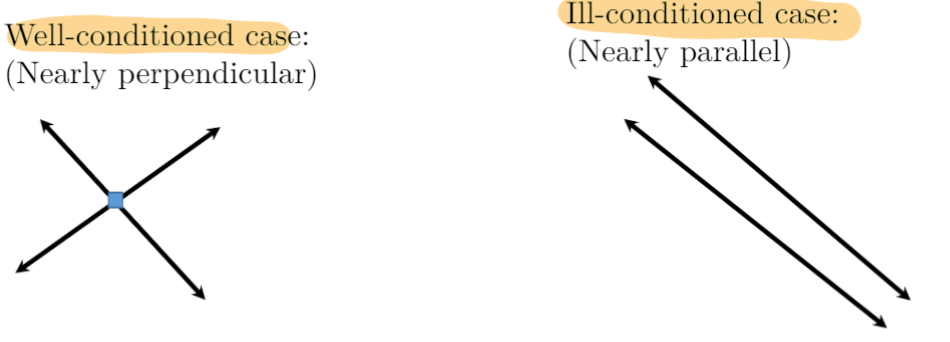
Well-conditioned case: Nearly perpendicular lines
Ill-conditioned case: Nearly parallel lines

Condition Number Summary

Condition number of a matrix $A$ is denoted $\kappa (A)=\parallel A\parallel \cdot \parallel A^{-1}\parallel$

1. $\kappa \approx 1⟹A$ is well-conditioned
2. $\kappa \gg 1⟹A$ is ill-conditioned
   For system $Ax=b,\kappa (A)$ provides upper bounds on relative change in $x$ due to relative change in $b$

or in $A$

$\kappa$ Depends on the Norm

We defined the condition number as

without specifying which norm. Different norms will give different $\kappa$
We can specify the norm with a subscript, e.g., $$\kappa(A)_2=|A|_2\cdot|A^{-1}|_2$$
If unspecified, always assume the 2-norm

Equivalence of Norms

The norms we’ve looked at differ from one another by no more than a constant factor
That is$$C_1|x|_a\leq |x|b\leq C_2|x|_a$$
for constants $C_1,C_2$, and norms $\parallel \cdot {\parallel }_a$ and $\parallel \cdot {\parallel }_b$.

Numerical Solutions: Residuals and Errors

Condition number plays a role in understanding/bounding the accuracy of numerical solutions
If we compute an approximate solution $x_{approx}$, how good is it?

• we need the exact solution $x$ for comparison
• recall: relative error = $\frac{\parallel x-x_{approx}\parallel }{\parallel x\parallel }$

Residual

As a proxy for error, we often use the residual $r$:

i.e., by how much does out computed solution fail to satisfy the original problem?

• This we can compute easily!
• We know $A,b$ our computed $x_{approx}$

Residual vs Errors

Assuming $x_{approx}=x+\mathrm{\Delta }x,$ we have$$r = b-A(x+\Delta x)$$or $$A(x+\Delta X) = b - r$$($r$ looks just like a perturbation of $b$!)
So, applying our earlier bound using $\mathrm{\Delta }b=r$, we have$$\frac{|\Delta x|}{|x|}\leq \kappa(A)\frac{|r|}{|b|}$$

Interpreting this Bound

The solution’s relative error, $\frac{\parallel \mathrm{\Delta }x\parallel }{\parallel x\parallel }$ is bounded by the condition number times the relative size of residual $r$ with respect to $b$
Moral: If we (roughly) know $A$’s condition number, the computed residual indicates how large the error might be

• if $\kappa \approx 1$, a small residual indicates a small relative error
• But, if $\kappa$ is large, residual could still be small while error is quite large!
  • Again, this is independent of the algorithm used to compute $x_{approx}$

Use of the Residual - Iterative Methods

Many alternate algorithms for solving $Ax=b$ are called iterative

• Similar to PageRank, they iteratively improve a solution estimate
• Size of residual dictates when to stop

Gaussian Elimination & Error

In floating point, Gaussian elimination with pivoting on $Ax=b$ is quite stable and accurate

• GE’s numerical result $\hat{x}$ gives the exact solution to a nearby problem (i.e. with perturbed $A$)

where $\parallel \mathrm{\Delta }A\parallel =\parallel A\parallel {ϵ}_{machine}$
Again, applying our earlier bound gives

e.g. if $\kappa (A)={10}^{10}$ and ${ϵ}_{machine}={10}^{-16}$, then the relative error in $x$ is around ${10}^{-6}$, or around 6 accurate digits

Conditioning is algorithm-independent

Condition is a property of the problem itself

• not a property of a particular algorithm
• i.e., A system $Ax=b$ is well- or ill-conditioned, independent of how we choose to solve it
  Even an “ideal” numerical algorithm can’t guarantee a solution will small error if $\kappa \gg 1$