Interpolation & Splines

Interpolation

The basic problem of interpolation

Given a set of data points from an (unknown) function $y = p (x)$ , can we approximate $p$ ’s value at other points?

e.g. Given $p (x_{1}) = y_{1}, p (x_{2}) = y_{2}, \dots, p (x_{n}) = y_{n}$
Estimate $y = p (x)$ for any point $x$ such that $x_{1} \leq x \leq x_{n}$

Theorem (Unisolvence Theorem)

Given $n$ data pairs $(x_{i}, y_{i}), i = 1, \dots, n$ with distinct $x_{i}$ , there is a unique polynomial $p (x)$ of degree $\leq n - 1$ that interpolates the data.

Vandermonde Matrices

Pasted image 20250302203411.png
$V$ is called a Vandermonde matrix

Polynomial interpolation reduces to solving systems of equations

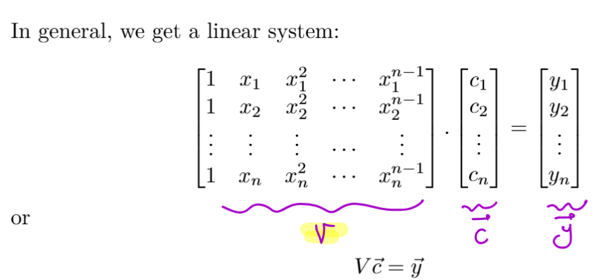
The monomial basis

The familiar form $p (x) = c_{1} + c_{2} x + c_{3} x^{2} + \dots + c_{n}^{n - 1}$ is called the monomial form, and can also be written as

p (x) = \sum_{i = 1}^{n} c_{i} x^{i - 1}

The sequence, $1, x, x^{2}, \dots$ is called the monomial basis.
Monomial form is a sum of coefficients $c_{i}$ times basis functions $x^{i}$ .

The Lagrange basis

We will define the Lagrange basis functions, $L_{i} (x)$ , to construct a polynomial as

p (x) = y_{1} L_{1} (x) + y_{2} L_{2} (x) + \dots + y_{n} L_{n} (x) = \sum_{i = 1}^{n} y_{i} L_{i} (x)

where $y_{i}$ are the coefficients and also our data values, $y_{i} = p (x_{i})$ .

Given $n$ data points $(x_{i}, y_{i})$ , we define

L_{i} (x) = \frac{(x - x_{1}) \dots (x - x_{i - 1}) (x - x_{i + 1}) \dots (x - x_{n})}{(x_{i} - x_{1}) \dots (x_{i} - x_{i - 1}) (x_{i} - x_{i + 1}) \dots (x_{i} - x_{n})}

When $i = j$ , $L_{i} (x_{j})$ has same numerator and denominator.
When $i \neq j$ , $L_{i} (x_{j})$ has numerator = 0, denominator $\neq 0$
Ensures $p (x)$ must interpolate each $x_{i}$

$p (x_{i}) = y_{i}$ by construction

Monomial vs Langrangian basis

They give the same interpolating polynomial
We can directly write down the polynomial from the Lagrange basis functions
No need to solve a linear system

Polynomial Interpolation for many points

Fitting a “high degree” ( $n \approx 7, 8, 9$ ) polynomial often gives excessive oscillation

Runge’s phenomenon

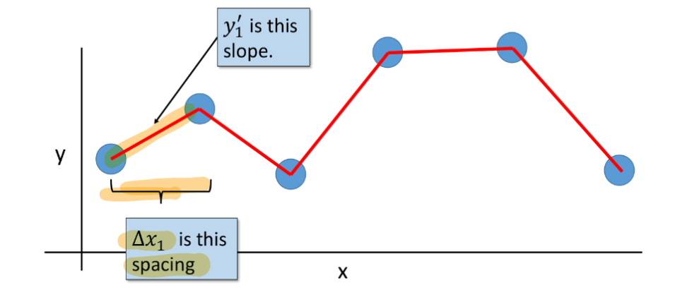
Piecewise Interpolation

Hermite Interpolation

The problem of fitting a polynomial given function values and derivatives

Closed-form Solution

Defining the polynomial on the $i^{t h}$ interval, $p_{i} (x)$ , as

p_{i} (x) = a_{i} + b_{i} (x - x_{i}) + c_{i} (x - x_{i})^{2} + d_{i} (x - x_{i})^{3}

We saw that the direct formulas for the polynomial coefficients are:

a_{i} = y_{i}, b_{i} = s_{i}, c_{i} = \frac{3 y_{i}^{'} - 2 s_{i} - s_{i + 1}}{Δ x_{i}}, d_{i} = \frac{s_{i + 1} + s_{i} - 2 y_{i}^{'}}{Δ x_{i}^{2}}

where we define

Δ x_{i} = x_{i + 1} - x_{i}

and

y_{i}^{'} = \frac{y_{i + 1} - y_{i}}{Δ x_{i}}

Pasted image 20250302214032.png

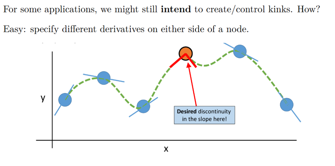
Some Terminology

Knots: Points where the interpolant transitions from one polynomial/interval to another
Nodes: Points where some control points/data is specified

For Hermite interpolation, these are the same
For other curve types (e.g. Bezier Curves), they can differ

More common problem: no derivative information

s_{i}

is given, only values

y_{i}

Can we still fit a piecewise cubic to the set of points?

Yes, but each “piece” needs data from more than just its 2 endpoints

Cubic Splines

Fit a cubic, $S_{i} (x)$ , on each interval, but now require matching first and second derivatives between intervals.
Require interpolating conditions on each interval $[x_{i}, x_{i + 1}]$ ,

S_{i} (x_{i}) = y_{i}, S_{i} (x_{i + 1}) = y_{i + 1}

and derivative conditions at each interior point $x_{i + 1}$

S_{i}^{'} (x_{i + 1}) = S_{i + 1}^{'} (x_{i + 1}), S_{i}^{″} (x_{i + 1}) = S_{i + 1}^{″} (x_{i + 1})

Counting Unknowns

Assuming $n$ data points, we have $4 (n - 1)$ unknowns

4 unknowns for each of $n - 1$ intervals

Counting Equations

Assuming $n$ data points, we have $2 (2 n - 3)$ equations

2 interpolating conditions per interval: $2 (n - 1)$
2 derivative conditions per interior point: $2 (n - 2)$

4 n - 6

equations,

4 n - 4

unknowns, can we solve the system?

No! Not enough information for unique solution!
Need 2 more equations

Usually at domain endpoints
Boundary conditions or end conditions

Boundary Conditions

Clamped

Slope set to specific value

$S^{'} (x_{1}), S^{'} (x_{n})$ specified
If both boundaries clamped, it is a complete or clamped spline

Free/natural/variational

S^{″} (x_{1}) = S^{″} (x_{n}) = 0

If both boundaries are free, called a natural cubic spline.

Curve “straightens out”

Periodic boundary

$S^{'} (x_{1}) = S^{'} (x_{n}), S^{″} (x_{1}) = S^{″} (x_{n})$
Start and end derivates match each other

“Not-a-knot” boundary conditions

Match 3rd derivates on end segments
- $S_{1}^{‴} (x_{2}) = S_{2}^{‴} (x_{2}), S_{n - 2}^{‴} (x_{n - 1}) = S_{n - 1}^{‴} (x_{n - 1})$
- Last two segments on an end become the same polynomial

Hermite vs. Cubic Splines

Hermite Interpolation: each interval can be found independently
Cubic Spline: must solve for all polynomials together at once!

Basic cubic spline approach

For $n$ points, we have $n - 1$ intervals / cubic polynomials, so $4 n - 4$ unknowns.
Write down:

$2 (n - 1)$ interpolating conditions: match inputs at interval endpoints
$n - 2$ first derivative conditions: match first derivatives at interior nodes
$n - 2$ second derivative conditions: match second derivatives at interior nodes
Additional boundary conditions for the 2 ends
Solve linear system of $4 n - 4$ equations for all polynomial coefficients

Cubic Splines via Hermite Interpolation

Use Hermite interpolation as a stepping stone to build a cubic spline!

Express unknown polys with closed form Hermite equations
Treat the $s_{i}$ as unknowns
Solve for $s_{i}$ that gives continuous 2nd derivates
Given $s_{i}$ , plug into closed form Hermite equations to recover poly coefficients.

Efficient Splines Summary

Interior nodes $(i = 2, \dots, n - 1)$ :

Δ x_{i} s_{i - 1} + 2 (Δ x_{i - 1} + Δ x_{i}) s_{i} + Δ x_{i - 1} s_{i + 1} = 3 (Δ x_{i} y_{i - 1}^{'} + Δ x_{i - 1} y_{i}^{'})

where we define

Δ x_{i} = x_{i + 1} - x_{i}

and

y_{i}^{'} = \frac{y_{i + 1} - y_{i}}{Δ x_{i}}

Clamped BC:

s_{1} = s_{1}^{*}, s_{n} = s_{n} *

Free BC:

s_{1} + \frac{s_{2}}{2} = \frac{3}{2} y_{1}^{'}, \frac{s_{n - 1}}{2} + s_{n} = \frac{3}{2} y_{n - 1}^{'}

Matrix Form

We can write this linear system for the slopes in matrix/vector form
Pasted image 20250303081103.png
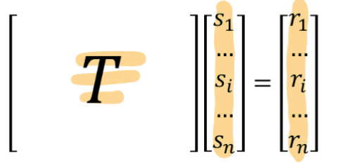
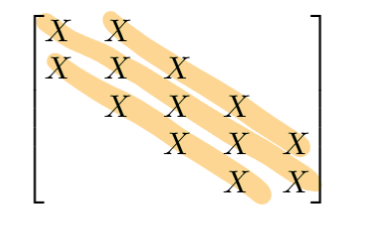
New system has one equation per node, no matrix size is $n \times n$ . This system is smaller in size by a constant factor 4.

Matrix Structure

The matrix is tridiagonal. Only the entries on the diagonal and its two neighbours are ever non-zero!
Pasted image 20250303081502.png

Shortcomings So Far

Cannot handle curve that has different $y$ for same $x$ .
Pasted image 20250303081735.png

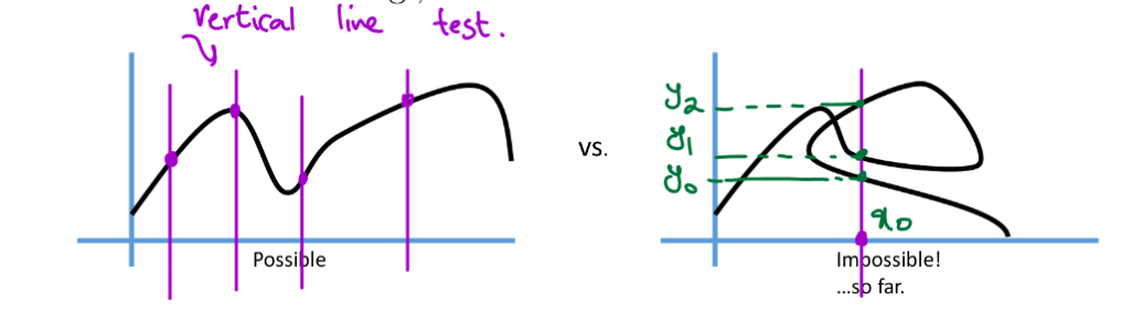
Parametric Curves

Lets us handle more general curves

Cannot express as $y = p (x)$

Solution

Let $x$ and $y$ each be separate functions to a new parameter, $t$ .
Then a point’s position is given by the vector $\vec{P (t)} = (x (t) . y (t))$ .
Pasted image 20250303082110.png
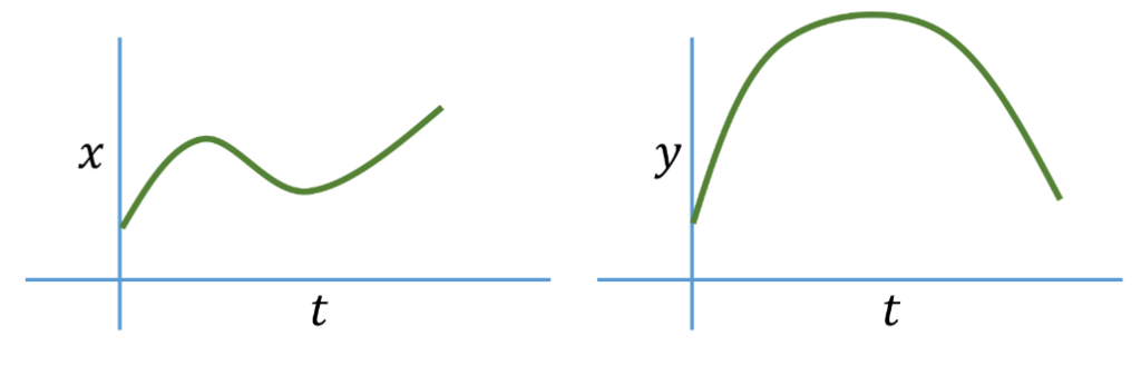
Parameter $t$ increases monotonically along the curve, but $x$ and $y$ may increase and decrease as needed to describe any shape.

Parametric curves are a more powerful/flexible way of describing curves in general

Non-Uniqueness

A given curve can be “parameterized” in different ways, while yielding the exact same shape.

Can traverse $t$ in opposite direction

Speeds

2 parameterizations can also traverse the curve in the same direction, but at different speeds/rates

Repeated Points

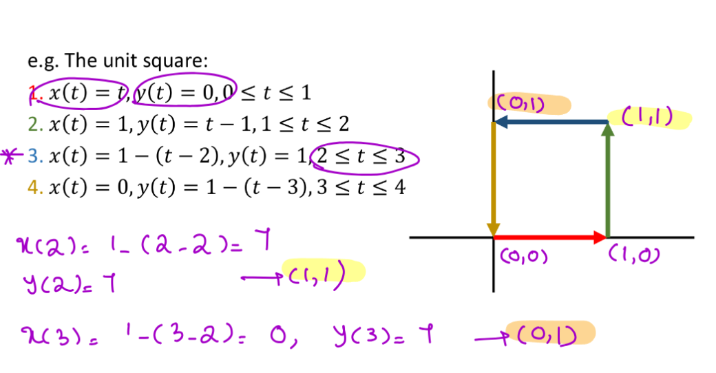
Curves with self-intersections are supported easily

Piecewise Parametric Curves

The unit square

Pasted image 20250303082910.png

Arc-Length Parameterization

Common to choose $t$ as the distance along the curve
Pasted image 20250303083024.png
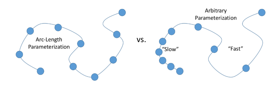
This gives unit speed traversal of the curve

Travel 1 unit of distance in 1 unit of time

Parametric Curves using Interpolation

Parametric curves are just the general concept
We can combine existing interpolant types with parametric curves by considering $x (t)$ and $y (t)$ separately

Use two Lagrange polynomials, $x (t), y (t)$ , to fit small set of $(t_{i}, x_{i}, y_{i})$
use Hermite interpolation for $x (t), y (t)$ given $(t_{i}, x_{i}, y_{i}, s x_{i}, s y_{i})$
Fit separate cubic splines to $x (t), y (t)$ , given many points

Parameterizations for Piecewise Polynomials

Given ordered $(x_{i}, y_{i})$ point data, we don’t yet have a parameterization.

We need data for $t$ , to form $(t_{i}, x_{i})$ and $(t_{i}, y_{i})$ pairs to fit curves to
Option 1: Use node index $i$ as the parameterization
Option 2: Approximate arc-length parameterization
set $t_{1} = 0$ at first node
Recursively compute $t_{i + 1} = t_{i} + \sqrt{(x_{i + 1}^{2} - x_{i})^{2} + (y_{i + 1}^{2} - y_{i})^{2}}$
- Distance between $(x_{i}, y_{i})$ and $(x_{i + 1}, y_{i + 1})$