Fourier Analysis

Fourier Transforms Introduction

The Fourier Transform applies to continuous functions or discrete data can provide useful insights and tools for many applications

Examples:
- signal processing
  - filtering
  - denoising
- sound/audio manipulation

Basic Idea

Transform some function/data into a form that reveals frequencies of information in the data
Process/analyse it it in this “frequency domain” form
Transform back again
The original data/function is said to be in the…

“time domain” if $f$ is a function of time, $f (t)$
“spatial domain” if $f$ is a function of space/position, $f (x)$

Convert time or space-dependent data into the representation

$f (t) = a_{0} + a_{1} \cos (q t) + b_{1} \sin (q t) + a_{2} \cos (2 q t) + b_{2} \sin (2 q t)$

i.e. infinite sum of increasingly high frequency sine/cosines
Could view this as:

a weird (non-polynomial) interpolation problem:
- what coefficients let us fit the particular summation form to a given function?
an expansion/approximation of the function as an infinite sum of sines/cosines
- e.g. compare to Taylor series

Main topics:

How do we find the coefficients for this frequency-based representation?
What if our input data are discrete values: $f_{0}, f_{1}, f_{2}, \dots, f_{N}$ instead of a smooth continuous function $f (t)$
- Discrete Fourier Transform, DFT
How can we transform data into the frequency-domain efficiently
- Fast Fourier Transform, FFT

Continuous Fourier Series

Consider some continuous periodic function $f (t)$ with period $T$ , so$$f(t\pm T) = f(t)$$i.e., $f$ repeats after one length/period $T$ .
e.g. $\sin (\frac{2 π k t}{T})$ or $\cos (\frac{2 π k t}{T})$ satisfy this for all integers $k$

\cos (\frac{2 π k (t + T)}{T}) = \cos (\frac{2 π k t}{T} + 2 k π) = \cos (\frac{2 π k t}{T})

Goal is to represent any $f (t)$ as an infinite sum of trig functions:$$f(t) = a_0 + \sum_{k=1}^{\infty}a_k\cos(\frac{2\pi kt}{T})+\sum_{k=1}^{\infty}b_k\sin(\frac{2\pi kt}{T})$$ $a_{k}, b_{k}$ indicate the ”information”/amplitude for each sinusoid of a specific period $\frac{T}{k}$ or frequency $\frac{k}{T}$

Higher integer $k$ indicates shorter period & higher waver frequency

Determining the Coefficients

Assume for now that $t \in [0, 2 π]$ and period $T = 2 π$
Then we have$$f(t) = a_0 + \sum_{k=1}^{\infty}a_k\cos(kt)+\sum_{k=1}^{\infty}b_k\sin(kt)$$

Handy Identities (Orthogonality)

\int_{0}^{2 π} \cos (k t) \sin (j t) d t = 0 for any integers k, j

i.e. the integral of the product of $\cos (k t)$ and $\sin (j t)$ over $[0, 2 π]$ is 0.
We say these two functions are orthogonal to each other

More Orthogonality Relations

\int_{0}^{2 π} \cos (k t) \cos (j t) d t = 0 for k \neq j

\int_{0}^{2 π} \sin (k t) \sin (j t) d t = 0 for k \neq j

\int_{0}^{2 π} \sin (k t) d t = 0

\int_{0}^{2 π} \cos (k t) d t = 0

We can use these to extract a single Fourier coefficient at a time!

Example

Determining coefficient $a_{0}$

We want $$f(t) = a_0 + \sum_{k=1}^{\infty}a_k\cos(kt)+\sum_{k=1}^{\infty}b_k\sin(kt)$$Integrate over $[0, 2 π]$ to use some of our orthogonality identities:

\int_{0}^{2 π} f (t) d t = a_{0} \int_{0}^{2 π} d t + \sum_{k = 1}^{\infty} a_{k} \int_{0}^{2 π} \cos (k t) d t + \sum_{k = 1}^{\infty} b_{k} \int_{0}^{2 π} \sin (k t) d t

Therefore:

a_{0} = \frac{\int_{0}^{2 π} f (t) d t}{\int_{0}^{2 π} d t} = \frac{1}{2 π} \int_{0}^{2 π} f (t) d t

i.e., $a_{0}$ is the average value of $f$ over $[0, 2 π]$

Determining coefficient $a_{l}$ (for integer $l > 0$ )

Again start with$$f(t) = a_0 + \sum_{k=1}^{\infty}a_k\cos(kt)+\sum_{k=1}^{\infty}b_k\sin(kt)$$Multiply by $c o s (l t)$ and integrate over $[0, 2 π]$

\int_{0}^{2 π} f (t) \cos (l t) d t = \int_{0}^{2 π} a_{0} \cos (l t) d t + \sum_{k = 1}^{\infty} a_{k} \int_{0}^{2 π} \cos (k t) \cos (l t) d t + \sum_{k = 1}^{\infty} b_{k} \int_{0}^{2 π} \sin (k t) \cos (l t) d t

The result is 0 except when $k = l$ . Hence, $$\int_0^{2\pi}f(t)\cos(lt)dt =a_l\int_0^{2\pi}\cos^2(lt)dt=a_l\pi$$
Thus, $$a_l = \frac{1}{\pi}\int_0^{2\pi}f(t)\cos(lt)dt$$

Summary

So if we have $f$ , we can find all the coefficients by solving integrals

a_{0} = \frac{\int_{0}^{2 π} f (t) d t}{\int_{0}^{2 π} d t} = \frac{1}{2 π} \int_{0}^{2 π} f (t) d t

a_{k} = \frac{\int_{0}^{2 π} f (t) \cos (k t) d t}{\int_{0}^{2 π} \cos^{2} (k t) d t} = \frac{1}{π} \int_{0}^{2 π} f (t) \cos (k t) d t

b_{k} = \frac{\int_{0}^{2 π} f (t) \sin (k t) d t}{\int_{0}^{2 π} \sin^{2} (k t) d t} = \frac{1}{π} \int_{0}^{2 π} f (t) \sin (k t) d t

How does phase of the sinusoids come in?

A sine is a translated cosine! All “in-between” shifts are just linear combinations of sin/cos

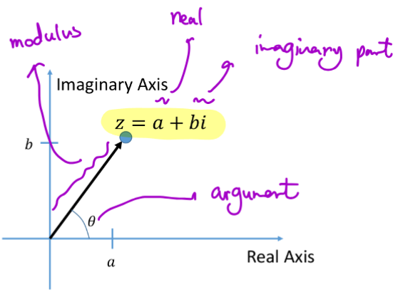
Complex Number Review

For $z \in C$ , we write $z = a + b i$ where the imaginary number $i = \sqrt{- 1}$
Visualized as points on the complex plane $(a, b)$ :

The vector length and angle are often called modulus and argument respectively

For $z = a + b i$ , we can define additional operations
Conjugate: $\bar{z} = a - b i$
Modulus/norm: $| z | = \sqrt{a^{2} + b^{2}}$
Argument/phase/angle: $A r g (z) = a \tan 2 (b, a)$
- converts rectangular coordinates $(x, y)$ to polar $(r, θ)$

Using Euler’s Formula

We will find Euler’s formula very useful:

e^{i θ} = \cos (θ) + i \sin (θ)

Also$$e^{-i\theta} = \cos(-\theta) + i\sin(-\theta) = \cos(\theta)-\sin(\theta)$$Adding/subtracting these lead to two key identities:

\cos (θ) = \frac{e^{i θ} + e^{- i θ}}{2}

\sin (θ) = \frac{e^{i θ} - e^{- i θ}}{2}

Fourier Series with Complex Exponentials

Now, given our earlier sinusoidal expression of a function $f (t)$ $$f(t) = a_0 + \sum_{k=1}^{\infty}a_k\cos(kt)+\sum_{k=1}^{\infty}b_k\sin(kt)$$we can express it more concisely as$$f(t)=\sum_{k=-\infty}^{+\infty}c_ke^{ikt}$$where the $c_{k}$ coefficients are complex numbers
There exists a simple conversion: $c_{k} ⟺ a_{k}, b_{k}$

Specifically for $k > 0$ :$$a_0=c_0, c_k = \frac{a_k}{2}-\frac{ib_k}{2}, c_{-k}=\frac{a_k}{2}+\frac{ib_k}{2}$$And we have the relationships:$$|a_0|=|c_0|,;\text{and };|c_k|=|c_{-k}|=\frac{1}{2}\sqrt{a_k^2+b_k^2}$$

Finding $c_{k}$ coefficients

We can also find $c_{k}$ directly, similar to what we did for $a_{k}$ and $b_{k}$
The corresponding orthogonality property is:$$\int_0^{2\pi}e^{ikt}e^{-ikt}=\begin{cases}0; k\neq l\2\pi; k=l\end{cases}$$from which we can determine the coefficient formula,$$c_k=\frac{1}{2\pi}\int_0^{2\pi}e^{-ikt}f(t)dt$$

Truncating

An approximation of a function could be achieved by truncating the series to a finite number of sinusoids:$$f(t)\approx\sum_{k=-M}^{+M}c_ke^{ikt}$$

Discrete Input Data

Consider now a vector of discrete data

e.g. $f_{0}, f_{1}, f_{2}, \dots, f_{N - 1}$ for $N$ uniformly spaces data points ( $N$ assumed even)
Assume data are from an unknown function $f (t)$ , evaluated at each
$t_{n} = n Δ t = \frac{n T}{N}$ , for $n - 0, 1, \dots, N - 1$
i.e. $f_{n} = f (t_{n})$

DFT as Interpolation

We have $N = 128$ points, and period $T = 32$
For $N$ points, we will use $N$ degrees of freedom (i.e $N$ coefficients) to exactly interpolate the data
Assuming $N$ is even, we can approximate with a truncated Fourier series as:

f(t)\approx\sum_{-\frac{N}{2}+1}^{N/2}c_ke^{\frac{(2\pi i)kt}{T}}$$If $T=2\pi$, then we will have the simplified version of it as $f(t)\approx\sum_{-\frac{N}{2}+1}^{N/2}c_ke^{ikt}$ Plugging in each of our $N$ data points $(t_n, f_n)$ into the expression will give us $N$ **equations**, involving **unknowns coefficients, $c_k$** This will lead towards our Discrete Fourier Transform ## Discrete Fourier Transform For notational convenience we defined:$$W = e^{\frac{2\pi i}{N}}$$$W$ is an **$N$th Root of Unity**, since it satisfies$$W^N = e^{2\pi i} = 1$$So$$f_n = \sum_{k=0}^{N-1}F_ke^{i(\frac{2\pi n k}{N})} = \sum_{k=0}^{N-1}F_kW^{nk}$$Discrete data $f_n$ is expressed as a sum of coefficient, $F_k$, times complex exponentials, $W^{nk}$ ### Roots of Unity With $W = e^{\frac{2\pi i}{N}}$, then  $$W^k = e^{\frac{2\pi ik}{N}}$$are also **Nth roots of unity,** for all integers $k$ For example: * for $N=3$, the roots of unity have the form $W^k = e^{k(\frac{2\pi i}{3})}$ * for $N=8$, the roots of unity have the form $W^k = e^{k(\frac{2\pi i}{8})}=e^{k\frac{i \pi}{4}}$ #### Complex Plane ![Pasted image 20250422165915.png](/img/user/assets/Pasted%20image%2020250422165915.png) **Each Nth root** corresponds to a point on the unit circle, in the complex plane Let $\theta = \frac{2\pi k}{N}$, then$$W_k = e^{i\theta} = \cos\theta + i\sin\theta$$Modulus is always 1, since $\sqrt{\cos^2\theta + \sin^2\theta} = 1$ ### Discrete Fourier Transform To be useful, operations we need are: 1. Convert input time-domain data $f_n$ to frequency-domain $F_k$ 2. Convert **frequency-domain data $F_k$** back to time-domain $f_n$ We derived#2; given Fourier coefficients $F_k$, we have: $$f_n = \sum_{k=0}^{N-1}F_kW^{nk}

What about #1? How can we solve for the $F_{k} = ? ? ?$

Another Orthogonality Idea

To find $F_{k}$ , we’ll need another useful property of our Nth roots of unity:

\sum_{j = 0}^{N - 1} W^{j k} W^{- j l} = \sum_{k = 0}^{N - 1} W^{j (k - l)} = N δ_{k, l} $ $ a s s u m i n g (f o r n o w) t h a t $ k, l \in [0, N - 1] $ T h e s y m b o l $ δ_{k, l} $ i n d i c a t e s t h e * * K r o n e c k e r d e l t a * * f u n c t i o n d e f i n e d b y : $ $ δ_{k, l} = {\begin{cases} 0; k \neq l \\ 1; k = l \end{cases}

A Discrete Fourier Transform (DFT) pair

Inverse DFT:$$f_n = \sum_{k=0}^{N-1}F_kW^{nk}$$
DFT:$$F_k=\frac{1}{N}\sum_{n=0}^{N-1}f_nW^{-nk}$$The Discrete Fourier Transform is invertible

Two Properties of the DFT

As consequences of the properties of Nth roots of unity…

The sequence ${F_{k}}$ is doubly infinite and periodic
- i.e. If we allow $k < 0$ or $k > N - 1$ , the $F_{k}$ coefficients repeat
Conjugate symmetry: if data $f_{n}$ is real, $F_{k} = \overset{―}{F_{N - k}}$
Hence, the $| F_{k} |$ are symmetric about $k = \frac{N}{2}$

Power/ Fourier Spectrum

The power spectrum visualizes the Fourier coefficients by plotting their moduli/magnitudes $| F_{k} |$ :
Pasted image 20250422183354.png
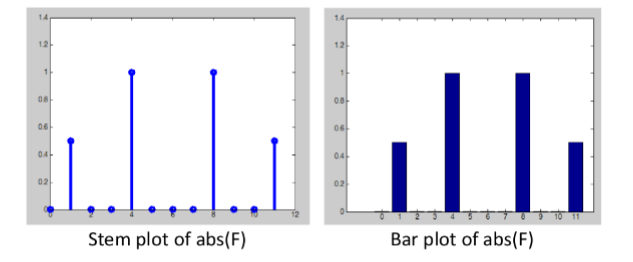
This expresses the magnitude of the frequencies, but ignores phase

Discrete Data - Observations

Coefficient $F_{0}$ is always the average of data values, $F_{0} = \frac{1}{N} \sum_{n = 0}^{N - 1} f_{n}$

sometimes called the direct current or DC

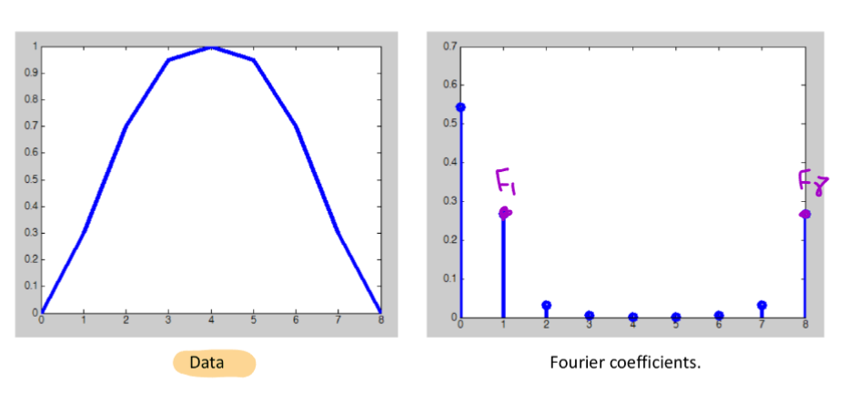
The smooth bump had one dominant frequency/wave; therefore one coefficient pair, $F_{1}$ and $F_{8}$ , had large magnitude

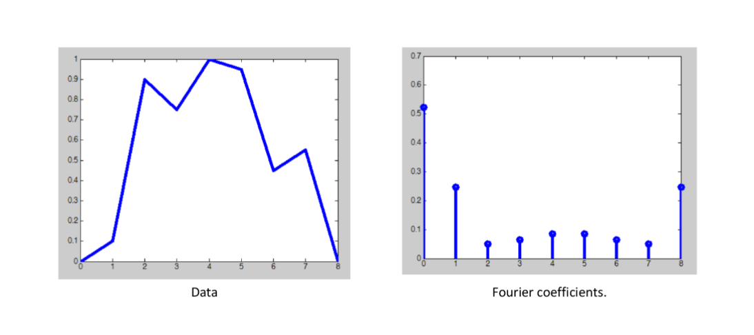
The rough bump had more irregularity, so more active (higher) frequencies.
Main hump still dominates, so low frequencies $F_{1}$ and $F_{8}$ remain largest

The Fourier $(F_{k})$ plots are symmetric, since the data was real

Fast Fourier Transform

Making Fourier Transforms Fast

Questions:

What is the complexity of the naïve method?
What property of the DFT allows it to be sped up?
How can we construct an algorithm from this property?
What is the complexity of the new method?

Slow Fourier Transform

A direct implementation of $F_{k} = \frac{1}{N} \sum_{n = 0}^{N - 1} f_{n} W^{- n k}$ takes $O (N^{2})$ complex floating-point operations
Essentially two nested for loops:
Pasted image 20250422185249.png

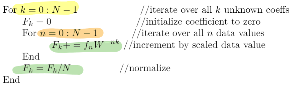
A Faster Fourier Transform

Design a divide and conquer strategy

Split the full DFT into two DFT’s of half the length
Repeat recursively
Finish at the base case of individual numbers
(If $N \neq 2^{m}$ for some $m$ , we can pad our initial data with zeros)

Dividing it up

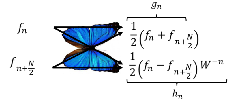
We can express the usual DFT with two new arrays of half the length ( $N / 2$ ):

g_{n} = \frac{1}{2} (f_{n} + f_{n + \frac{N}{2}}) $ $ $ $ h_{n} = \frac{1}{2} (f_{n} - f_{n + \frac{N}{2}}) W^{- n}

where $n \in [0, \frac{N}{2} - 1]$ .
Then, $F_{e v e n} = G = D F T (g)$ and $F_{o d d} = D F T (h)$ .

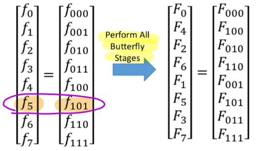
Visualizing - A Butterfly Operation

We can think of each step as taking a pair of numbers and producing two outputs:
Pasted image 20250422190321.png

Big Picture - Recursive Butterfly FFT Algorithm

Pasted image 20250422190428.png
$N = 8 = 2^{3}$ , so we have 3 recursive stages
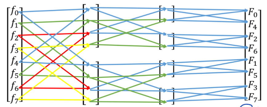
Note: Coefficient output order is scrambled
Pasted image 20250422190751.png

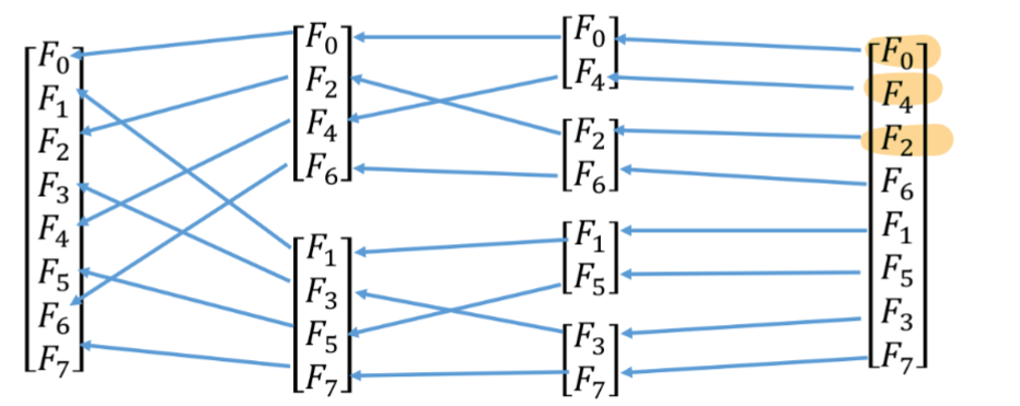
Each step applies an even-odd index splitting for the result location. So, the output ends up in bit-reversed positions

Is it actually faster?

We spend $O (N)$ operations to split the arrays in two, at each stage
Data has length $N = 2^{m}$ , so we need m = $\log_{2} N$ stages
Total cost $O (N \log_{2} N)$ operations
- compared to $O (N^{2})$ of DFT

Inverse Fast Fourier Transform

Consider the generic expression: $$f'k=\frac{1}{N}\sum^{N-1}f_nU^{nk}$$If $U + W^{- 1}$ , this is our forward DFT

$U = W^{- 1}, f^{'} k = F_{k}, f_{n} = f_{n} \to F_{k} = \frac{1}{N} \sum_{n = 0}^{N - 1} f_{n} W^{- n k}$
If $U = W$ , and we post-multiply by $N$ , this is the inverse FFT
$U = W, f_{k}^{'} = f_{n}, f_{n} = F_{k} \to f_{n} = \sum_{k = 0}^{N - 1} F_{k} W^{n k}$

Fourier Application: Image Data/Compression

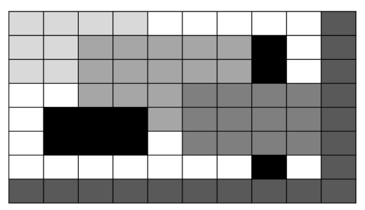
1D Grayscale Image

We can think of a 1D array of grayscale values as a 1D image

Each entry gives the pixels’ intensity/grey values

Processing 1D Images

For greyscale images, we can perform a DFT on the pixels’ intensity/grey values
Pasted image 20250422194813.png
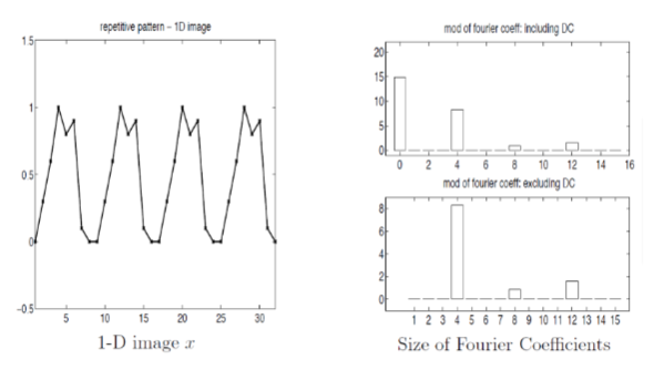
Notice: Plot is only the first 16 coefficients, since real data implies conjugate symmetry

Overall pattern has few coefficients active
- Can store it cheaply just with $F_{0}, F_{4}, F_{8}, F_{1} 2$
  If we destroyed the repetition (e.g. flat line top for the 3rd bump)
Many more Fourier coefficients will become active/non-zero
becomes expensive to store
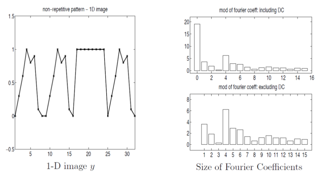
Although many coefficients are non-zero, many still have fairly small moduli/magnitude…
- so those frequencies contribute less to the image

Compression Strategy

Create an approximate compressed version of the image, $f_{n}$ , by throwing away small Fourier coefficients
- $| F_{k} | < t o l$
To reconstruct the image, run the inverse DFT to get modified data (pixels), ${\hat{f}}_{n}$
Discard the imaginary parts of ${\hat{f}}_{n}$ , to ensure new data is strictly real

Comparison

Pasted image 20250422195707.png
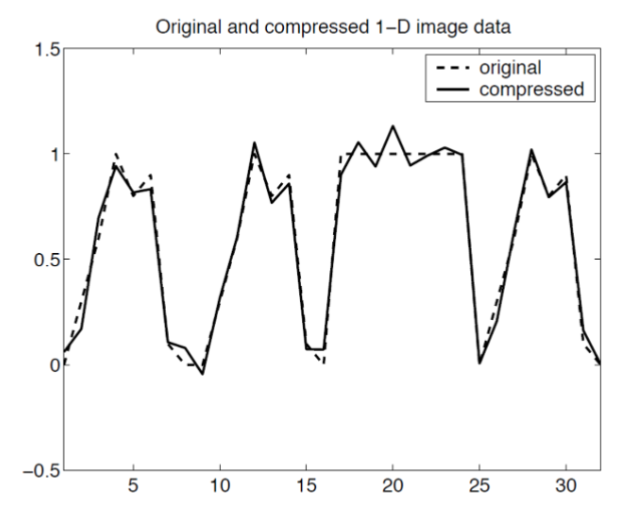
Recovered “image” hopefully has small deviations from the original “true” data

But! We store fewer Fourier coefficients and so save space!

Image Processing in 2D

Pasted image 20250422195824.png

How does the DFT work for 2D (greyscale) image data?

We apply a 2D extension of the DFT definition to the data, like so:

F_{k, l} = \frac{1}{N M} \sum_{n = 0}^{N - 1} \sum_{j = 0}^{M - 1} f_{n, j} W_{N}^{- n k} W_{M}^{- j l}

Essentially two standard (1D) DFT’s combined.
Two (possibly distinct) roots of unity are used, one per dimension:

W_{N} = e^{\frac{2 π i}{N}} and W_{M} = e^{\frac{2 π i}{M}}

Result is a 2D array of Fourier coefficients, $F_{k, l}$

2D Fast Fourier Transform

Pasted image 20250422200410.png
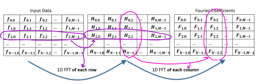
The 2D FFT can be computed efficiently using nested 1D FFTs:

Transform each row (separately) using 1D FFTs
Transform each column on the result, again using 1D FFTs

Complexity

Performing $M$ 1D FFT’s of length $N$ : $M \times O (N \log_{2} N) = O (M N \log_{2} N)$
Performing $N$ 1D FFT’s of length $M$ : $N \times O (M \log_{2} M) = O (M N \log_{2} M)$
So total complexity is $O (M N (\log_{2} M + \log_{2} N))$

Block-based Image Compression

Pasted image 20250422200752.png
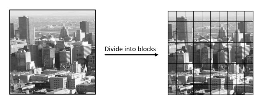
Often an image is subdivided into smaller blocks: $16 \times 16$ or $8 \times 8$ pixels

Compression is performed on each block independently
Idea: Pixels within a block often have similar/related data, and hopefully compress effectively

Fourier Application: Understanding Aliasing

Sampling of Signals: Aliasing

If a real input signal contains high frequencies, but the spacing of our discretely sampled data points is inadequate, aliasing can occur
Pasted image 20250422202037.png
A truly high frequency signal (red) aliases as a lower frequency signal (blue) in the discrete result

Takeaway

Our DFT coefficients $F_{k}$ are sums of true continuous Fourier series coefficients $c_{k}$ of increasing frequency:

F_{k} = c_{k} + c_{k + N} + c_{k - N} + c_{k + 2 N} + c_{k - 2 N} + \dots

Hence, high frequencies from $c_{k} \notin [- \frac{N}{2} + 1, \frac{N}{2}]$ in the real signal contribute to (“alias as”) low frequency $F_{k}$ for $k \in [- \frac{N}{2} + 1, \frac{N}{2}]$ .

Nyquist Frequency

If the original continuous signal has frequencies $c_{k} \neq 0$ for $| k | > \frac{N}{2}$ those frequencies “alias” to a lower frequency

Once a signal is discretely sampled, there is no way to distinguish aliased (high) frequencies from real (low) frequencies

Treating Aliasing

Two (partial) solutions:

Increase the sampling resolution to capture higher frequencies
Filter before sampling to remove (too) high frequencies
- so they don’t cause aliasing

Example:

Digital Cameras often have optical lowpass filters or anti-aliasing filters that physically blur the incoming light, before it hits the image sensor